I have data in on one cell like
columnA
VADODARA - 390010
KALWAKURTHY -509324
CHENNAI -600042
I need output like
columnA       columnB
VADODARA      390010
KALWAKURTHY   509324
CHENNAI       600042
Please tell me how to do this.

I have data in on one cell like
columnA
VADODARA - 390010
KALWAKURTHY -509324
CHENNAI -600042
I need output like
columnA columnB
VADODARA 390010
KALWAKURTHY 509324
CHENNAI 600042
Please tell me how to do this.
How about Data > Text to Columns, setting the Separator options to Separated by > Other - (hyphen)?
If trailing spaces on the text column cause problems, then do a search for spaces and replace with nothing.
I didnot get your answer can you show me with one example
@Ram.BM: select the cells with the data you want to split into columns and then click on the menu Data and follow the steps described by w_whalley
The needed formula is to be seen in the screenshot.
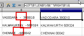
However, the formula requires that after the city name (any length of the citiy name is possible), there is blank followed by a hyphen, followed by a blank, followed by a 6 digit numercial or alphanumercial string. See also the red marks in the screen shot.
@ROSt53, that does not separate the data to two columns as requested. w_whalley’s answer does what was asked.
@Pedro1 - You are right. I somehow thought @Ram.BM wants to have all in one column with the hyphen. 2 colums makes it easier 1. colum: =left(b1,len(b1)-9 and 2. column: =right(b1,6)
@w_whalley’s idea with Text to Column looks also very good.