Count frequency of unique cell values in Calc

[Carlyle]

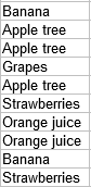
Let’s say I have a column with these entries:

I want a method that gives me this result:

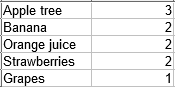
What I want is to list unique cell entries in the column and sort them by frequency.

Notes:

• Cells can have either a single word or multiple words as seen in the example (not sure if this is relevant to mention, but just in case).
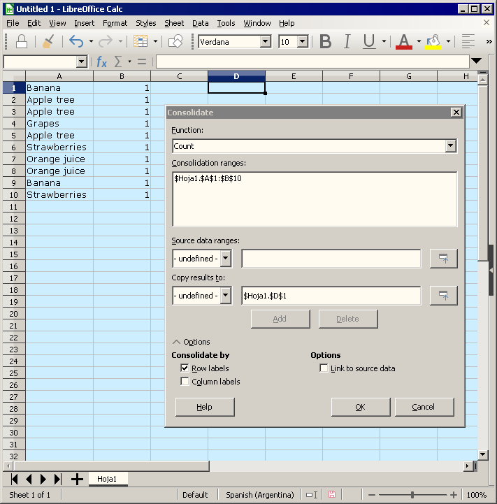
• I don’t know how many unique cell values there are, so I can’t use something like =COUNTIF(A1:A10;"Banana"). My column has over 1 million cells, so there are probably dozens of thousands of unique entries.
• It’s not necessary to list them all, I only need the 100 most frequent entries.

[Regina]

Your data need a first row with a label.

• Mark all data including the label and name it. That is in Data>Define Range. Make sure, that in part Options, the option Contains column labels is checked.
• Keep the range marked, or in case you lost the selection, use Data>Select Range to mark it again.
• Call the Pivot-Table wizard. That is an icon in the toolbar, or Data>Pivot Table.
• Drag your label from Available Fields: into the part Row Fields: and into the part Data Fields.
• Double-click the label in the part Data fields and select item Count.
• Make sure that the Pivot table is generated in a new sheet, because we will filter it later on. Find the setting in part Source and Destination. You do not need totals, so you should disable them in the part Options.
• Go to the Pivot table and select the entire table. A quick way for that is: Click into the Pivot table and press Strg+*(in the numpad).
• Then set a filter by Data>More Filters> Standard Filter. In field Field name select Count - your label. In field Condition select Largest and in field Value write 100. OK.

[jasom]

Your answer finally motivated me to create an account here. To the problem. Presented solution is either too complicated (I see you are from Germany :D) or the soft - Calc - needs to be improved. I thing well balanced conclusion is “20% engineering overkill, 80% Calc needs improvement”. See below my approach.

[jasom]

Scenario:

In the column A we have 20000+ of strings we want to count.

Remove duplicated using this tool (yes, even removing duplicates using Calc is insane complicated) and paste them (SHIFT + CTRL + V) to the column B.

In the column C use this formula: =COUNTIF($A$1:$A$20000;B1)

That’s it.

[jrussell88]

A quick way to remove duplicates in Column A is to sort by Column A, then enter a formula in Column B: =IF(A2=A1,"",1)

Every first occurence of an entry in Column A will be marked with ‘1’ in Column B; duplicates will be blank. Copy Column B, Paste Special - Numbers back to this column to replace the formula with its results.

Sort by Column B, and all the duplicates in A will be at the bottom of the column.

[LeroyG]

Carlyle,

Add a column with ones next to the entries.

Choose Data - Consolidate… Consolidate.png

If new column have ones, Function could be Sum or Count.

In Source data ranges: type A1:A10, then pulse Add.

In Copy results to: type the range where you wish the results.

Select Row labels.

Pulse Ok.

Then you can sort by frecuency.

LibreOffice Help on Combine Cell Contents.