How to find where in the interval a number is

Imagine we have 3 columns, the first two define a range (e.g. min and max weight) and the third the value (e.g. price that item costs if it has that weight).
Example

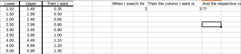
What formula should be used to achieve this?

From this site I was able to build something that returns the number of the column, but I would now need to get column C.
To get the column number I use =IF(SUMPRODUCT(–(A1:A39<=F2)(B1:B39>=F2))=1,SUMPRODUCT(–(A1:A39<=F2)(B1:B39>=F2),ROW(A1:A39))-1,“Not Found”)

here is an example file: How to find value corresponding to interval.ods - Google Drive

Questions:

  1. How would I retrieve the corresponding value in C?
  2. Is there an easier way to do this?

The world isn’t organized in steps of one hundredth.
Assume you intervals left side closed, right side open. The first row e.g. covering
1.10 <= value < 1.50, the next interval then being 1.50 <= value < 2.00.
If actually only occur values gtting integer when multiplied with 100 this won’t spoil anything.
Anyway the column of upper limits is superfluous.

I agree. The real world example actually is organised in steps of one hundredth (it is a cost and they don’t define less than one cent of euro), but I agree that from the calculation’s point of view the upper limit is not needed.

This is a cvase for one of the lookup variants. Since your lower limits are included with the respective intervals (left closed), you can use VLOOKUP() or a combination of MATCH() and INDEX() [or OFFSET()], both with the sort parameter 1 giving the assurance that the lower limits are strictly ascending top down.

(Edit1 regarding the comment below:)
Using VLOOKUP no additional checks are needed.

If the value to select the interval does not produce a match an eror will be returned. There are sufficient means to handle the situation without a need to check specifically for that value being a number.

I made this example preferring the flexible combination of MATCH() with INDEX(). (Even more flexibility is achieved using OFFSET() in some places.) The example values (now in column E instead of F) are mostly generated randomly.

How to alert users to enter valid entities was not my concern. If addressing this, I would prefer to use a conditional format.

For eg.

=VLOOKUP($F$2,$A$2:$C$10,3)

To check the range, perhaps use MIN() and MAX()

Ie,

=IF(MAX($A$2:$A$10)<$F$2,“Too Large”, IF(MIN($A$2:$A$10)>$F$2,“Too Small”,VLOOKUP($F$2,$A$2:$C$10,3)))

And to check that the F2 search value is a number, use ISNUM().

Ie,

=IF(ISNUM($F$2),IF(MAX($A$2:$A$10)<$F$2,“Too Large”, IF(MIN($A$2:$A$10)>$F$2,“Too Small”,VLOOKUP($F$2,$A$2:$C$10,3))),“Enter Number”)

This works really well, thanks!