Navigate to specific cells using Ctrl+arrow keys

Greetings All,

I regularly use Ctrl+downarrow to move to the next cell containing a value in columns in Calc.

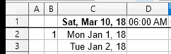
I made a diary recently.

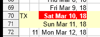
I used conditional formatting to highlight the current day in red, as shown in the lower image. Lovely.

I’d like to use Ctrl+downarrow to move to the current day, but of course I can’t because all the cells in that column (C) contain formulas and resultant values.

So, I made a formula that shows TX in column A if the value of the adjacent cell C == C1. You can see, for example, that C70 == C1 in the images. Again, just what I wanted.

When the sheet opened I tried using Ctrl+downarrow (in column A) to jump to A70 (the current day and the only cell showing TX).
The problem is that Ctrl+downarrow not only jumps to cells with displayed values, but also to cells containing formulas even though such cells aren’t displaying any values.

Effectively, it moves down to the last cell in column A containing a formula (A365 in this sheet) rather than to the next cell displaying a value (TX). Not what I wanted.

I’d like to find, or create, a key combination that moves to the next cell with a displayed value in column A and doesn’t include cells that display nothing but which contain formulas.


image description


image description

C1 contains =TODAY()

C2 contains 01/01/2018

C3 contains =C2+1 The remaining cells in column C continue to reference the cells above them.

A70 (and all the cells above and below it) contains =IF(C70=C$1,“TX”,"")

(The numbers in column B are just the manually entered week numbers, in case anyone was wondering)

Thanks in advance for any help offered.

Please don’t supply images with questions concerning the functionality inside documents. Attach a documant demonstrating the situation instead.

OK. First time here. I scanned the guidelines but I guess not thoroughly enough.

Quoting @PWT: “I’d like to find, or create, a key combination that moves to the next cell with a displayed value in column A and doesn’t include cells that display nothing but which contain formulas.

Theree isn’t such a shorcut - and you cannot set one, because the property “is blank or contains a formula currently returning the empty string (or just whitespace characters?)” is too complex to be supported by the queries running in the background if you pressed Ctrl+Arrow.

You would need to write a user Sub for the purpose and to asign it to your chosen shortcut.
If you can accept to have a similar functionality at hand only in specific cells (in the first frozen row e.g.), you may place a formula based on the HYPERLINK() function there. A subformula has to return the address of the target cell then, and HYPERLINK can provide the target for a jump by mouseclick (or Ctrl+mouseclick).

There was a related request in the German branch to which I supplied a working answer. If your German is sufficient, you may start with that proposal and adapt it to your needs.

Edit1:
See also this attachment.
The range is fix there. You should replace the fix upper limit for row numbers by a variable one used on the third parameter position of an OFFSET() sub-expression.

Greetings Lupp,

Thanks for your reply. It was most helpful, but oddly enough, not for this problem. As far as the difficulty outlined above is concerned, I simply changed the way I use the program and it works well enough. However I did look at the German link you included and although my German is non-existent, Google Translate worked well enough. I’ll use the methods shown there for something else I’m working on. Thanks for replying to my original query.