LOOKUP with linear interpolation for missing values

[endolith]

I have a table of data like this

0	-105.0
10	-114.3
20	-121.8
30	-127.0
40	-129.6
50	-130.8
60	-131.2

I’ve discovered the LOOKUP() function, which lets me input a value from the first column and returns a value from the second column. (=LOOKUP(20, A1:A7, B1:B7) returns -121.8, for instance.)

But is there a way to use linear interpolation to fill in the gaps between the samples? For example, a hypothetical =LERPLOOKUP(15, A1:A7, B1:B7) would return -118.07, the midpoint between the 10 and 20 values.

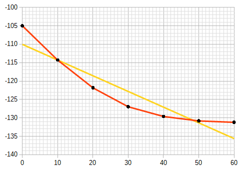
In other words, if the data is the black dots, it should find points along the red lines (linear interpolation), not along the yellow line (linear regression):

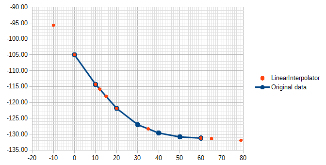
(and maybe linearly extrapolate outside the data, though that will be totally wrong for some data, and become increasingly wrong the further out you go.)

[ve3oat]

The question and all the answers are fascinating. Thank you.

[endolith]

I found a solution on an external website: Tarsier Tools Linear Interpolation Function

It uses a syntax very similar to my proposal (=LinearInterpolator($A$1:$A$7, $B$1:$B$7, 15)), and extrapolates outside of bounds, too.

It was a little difficult to get installed, probably because of macro security paranoia, but I put the downloaded file in a trusted folder and was then able to drag it from the document to my default macros folder.

[Regina]

I want to show you a solution using the widely unknown function MULTIPLE.OPERATIONS. MultipleOperations.ods

It is useful, if you need the same calculation very often. It can be written with one or with two arguments. The example in the attached document uses the version with one argument.

The basic idea is, that you make a template for the calculation. The calculation in the template can be made in several steps. That has the advantage, that the calculation is easier to understand and can be better maintained. It needs neither named expressions nor macros.

After you have made the template calculation, you can use it in the MULTIPLE.OPERATIONS function.

Syntax for one argument MULTIPLE.OPERATIONS(a;b;c)

a contains the cell address of the result cell of the template.

b contains the cell address, which is used for the argument in the template result formula.

c contains the cell address of the current, new value for the argument. A literal value is not possible.

Syntax for two arguments MULTIPLE.OPERATIONS(a;b;c;d;e)

a, b, c same as above

d contains the cell address, which is used for the second argument in the template result formula.

e contains the cell address of the current, new value for the second argument.

[gdgrosse]

Use of the built-in MULTIPLE.OPERATIONS() function is ideal as it does not require external untrusted macros to function.

Regina’s work here is very impressive.

Just finished implementing a refrigerant temperature to pressure lookup table interpolation.

The only limitation discovered after running many text cases inbounds and out of bounds is that it fails to handle the last value in the series.

This limitation can be worked around by manipulating your data to add one last entry to the series with a very small increment to the x value, for example if the last x value is 21.1, add a line to the series with an x value of 21.1000000001 and the same y value.

Regina, we would certainly apprecite it if you could resolve this limitation.

[mikekaganski]

=FORECAST.LINEAR(15;B1:B7;A1:A7) - but it seems to give different result (-116,418) - must have something to do with it specifically targeted at extrapolation

[endolith]

That looks like linear regression, not linear interpolation. So it fits a line to ALL of the points and then interpolates with that, rather than fitting a line to the nearest 2 points and interpolating between them.

[endolith]

Added an image to clarify