Gregors15 idea of the extra column really solved my problem I was having, so all the credit should go to Gregors15.
By adding a unique value to each row using the ID and Field column you can perform a lookup of the Value using a formula that uses INDEX and MATCH.
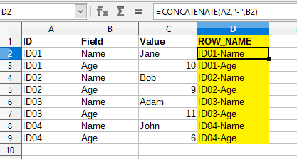
Step 1
Create a new column called “ROW_NAME” that joins the ID and Field column using the following formula
=CONCATENATE(A2,"-",B2)
Step 2
Rename current sheet “before”
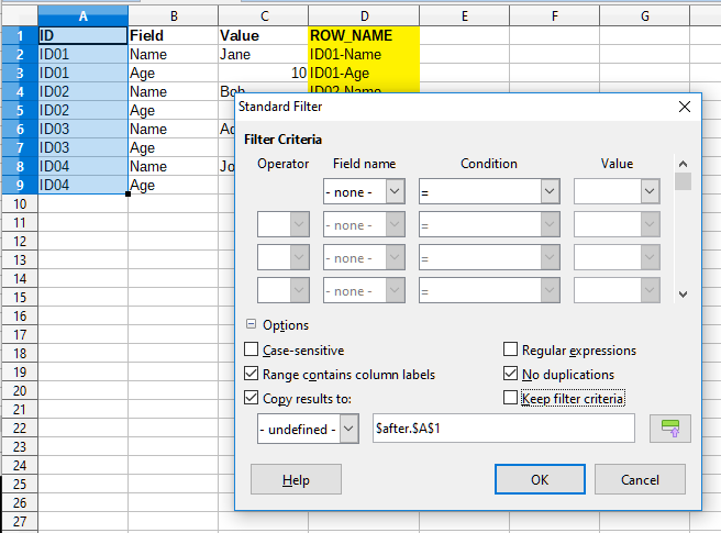
Step 3
Create a new sheet called “after” with distinct list of the ID column. Use the filter located in the menu “Data>More Filters>Standard Filter” (see the screenshot below how to configure the dialog box)
Step 4
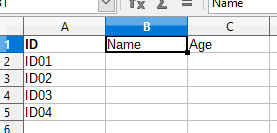
Capture the columns names you want starting at B1 on the “after” sheet
Step 5
Enter the following formula at B2 on the “after” sheet
=INDEX($before.$C$2:$C$5000,MATCH(CONCATENATE($A2,"-",B$1),$before.$D$2:$D$5000,0),0)
The formula works as follows it calculates the “ROW_NAME” value using the CONCATENATE($A2,"-",B$1) then it searches for it the range “$before.$D$2:$D$5000” and then the INDEX function returns the Value contained in the range “$before.$C$2:$C$5000” that is located at a row that the MATCH function found.
Step 6
Drag the cell to fill the sheet with calculation needed for each cell.
Here is the final document.solution.ods