Searching columns for data to return max value of adjacent column? [SOLVED]

[HawluchaTap]

This is quite the complex dilemma, so bear with me. I run a shop on a Pokemon fansite-type thing selling members of various Pokemon species that I’ve hunted, and I decided today to make a spreadsheet to better enable me to run that shop. The sheets I have made so far detail the current stock of my store, the order in which said stock should be displayed, the type distribution across my stock, and - the problem sheet - a list of future hunts to create future stock.

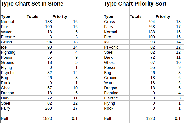
My Type Distribution page looks like this, currently. It totals the occurrence of each type across the previous page and then ranks them in descending order from highest quantity; said rank is hereafter called “Priority”.

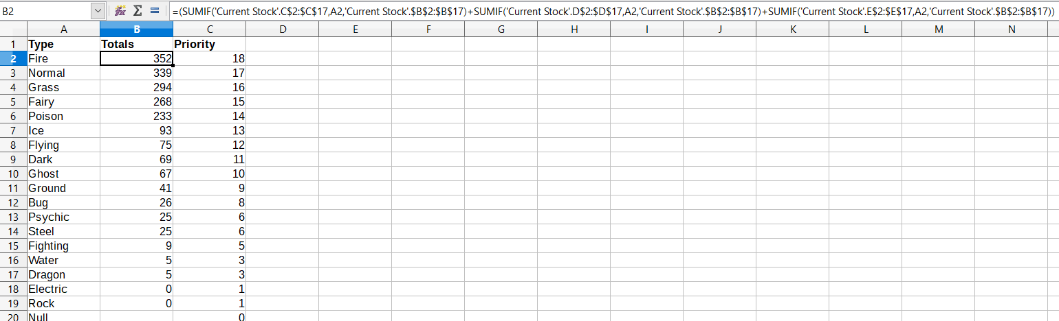
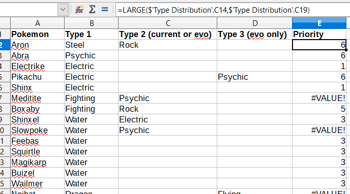
Here, meanwhile, is my current Future Hunt Priorities set-up. What I would like to achieve is to match the types of each Pokemon in Columns B-D against Columns A-C in the previous sheet, and return the highest number from Column C Sheet 2 in Column E Sheet 3. For example, if a Pokemon covers the types Bug, Flying and Steel in its lifetime, I would like the Priority column to return the highest Priority in the previous sheet out of those types.

(Don’t worry, the ‘blank’ cells in Sheet 3 aren’t really blank; they’re filled with the word Null that happens to be in white text so it’s not an eyesore but it still counts as observable data. This is why Null appears in Sheet 2 as well.)

As you can see, I attempted to recreate a facsimile of the formula by using the Large function to select the highest of two types manually selected. While it patches the gaps theoretically, I don’t see it being practical in the long term, because my stock levels are subject to change, and thus priorities will shift accordingly on Sheet 2 and the data on Sheet 3 will thus no longer be accurate. The ideal formula for this situation would be one that works regardless of the order of types and will always return the result two columns to the right of the matching data regardless of which row it’s in, but thus far I haven’t been able to find a formula that functions like this. I’ve also attempted the OFFSET formula, to no success.

I also enclose a download link of the spreadsheet in question, to see if anyone working manually with it may be able to divulge better results: http://www.mediafire.com/file/9zz39ucvh3r2lyf/pokefarm_store_sheets.ods

Thank you in advance! This is my first post, so let me know if there’s anything I need to clear up.

[gregors15]

Hi, have a look at the uploaded file, I have used index/match to find the priority for each Type, and then just used MAX to populate the Priority.
LO20190801.ods
Let us know if it helps.

[HawluchaTap]

Thank you very much, this does help! I had unfortunately already pseudo-engineered my own solution by the time you posted this, but I will keep this information in mind if I should need to tweak or streamline the spreadsheet or apply the techniques to something else in the future!

[HawluchaTap]

So I was working on this problem some more over the weekend, and here’s what I came up with independently. It actually uses a similar framework to gregors15’s solution, in that it relies on putting the types in more than one table, but the reasoning’s a little different.

What I ended up doing was taking my original Type Distribution table and duplicating it into a ‘Type Chart Set In Stone’ table and a ‘Type Chart Priority Sort’ table. This way, I had one where the order of the types would always be consistent, where the Psychic priority would always be in cell C14 etc, and one with the same or similar formula that I could sort to show highest or lowest priority as needed. It now looks thus:

(The numbers are only different because my stock has changed since the post.)

For the Future Hunt Priorities sheet, I then inadvertently used the same method as, again, gregors15 to populate the Priority: using =MAX to compare between multiple types (as =LARGE was repeatedly failing on types with the same priority, I found), and just displaying the corresponding cell for single-type species. I gave up on the Offset approach as it was repeatedly failing to show results, and with the table I was drawing from now in a set order I could just draw from the necessary cell directly.

As I said, I do appreciate gregors15’s contribution! That can’t have been easy for you to figure out either; and now I know that the =IF(ISBLANK(#)#) formula exists, which could prove VERY useful for further down the road. Either way, though, I’m going to go ahead and mark this one solved, because it’s got an answer from both ends of the questioner-responder spectrum now - the latter’s the one marked as correct, both because I’m a new user and cus they deserve that much.

Sorry for wasting your time!