Time average

I have a column of time spans. For example
8:45:06
12:35:45
etc

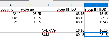
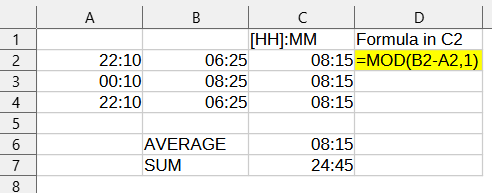
I’d like to determine the average time span. Like, what is the average amount of hours I spent doing X each day. Not what average time I started X (although I have that data) but time spent.

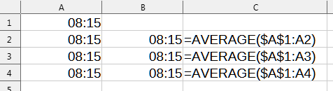
=AVERAGE(A1:A2) gives 0.

=AVERAGE(A1:A2)/24 gives #DIV/0! (read here about how spreadsheets see time as % of days vs hours)

=SUM((A1:A2)/2 gives 0 (this is the formula used for the other columns that are just numbers)

Numbers are formated as time 00:00:00 without the PM because it isn’t a clock time but an amount of time.

Surely I don’t have to do /24 for each entry. That would be time consuming. And I’d have to do another average listing. :wink:

Usually it’s matter of having the values as text. Select a couple of cells or the column, and use Menu/Data/Text to convert in true time values.

49901.ods (85.2 KB)

Just plain average worked for me with no trouble.

Maybe start fresh with the formats in case something got messed up? Use right-click > Clear Contents… > Formats on all your time cells, and then re-do the time formats. (Edit: if this is a large spreadsheet, maybe experiment with a small area first.) It sounds like you picked the correct ones, but if it helps here are the ones I used:

Format for A2:B4 - Category:Time, Format code HH:MM:SS AM/PM

Format for D2:D4 and D6 - Category:Time, Format code HH:MM:SS

        A               B           C                  D
1  Start time      Stop time     Formula            Result
2  04:00:00 PM     05:00:00 PM   =B2-A2             01:00:00
3  03:00:00 AM     10:00:00 AM   =B3-A3             07:00:00 
4  11:00:00 AM     01:00:00 PM   =B4-A4             02:00:00
5
6                  Average:      =AVERAGE(D2:D4)    03:20:00

The average of 1, 7, and 2 is 3.3333, so the result is correct.

Thanks! I’ll give that a try.

UPDATE: Libreoffice is not buggy, I was just unknowingly mixing positive and negative durations

Actually, libreoffice, unless it has been fixed (I’m using version 7.6), has trouble providing correct average for times.
Average of say 8:15 and 8:15 is as expected 8:15.
But average of say 8:15, 8:15 and 8:15 is not 8:15, but 0:15.
Perhaps it internally uses SUM(range) / COUNT(range). And SUM of 8:15, 8:15 and 8:15 is 0:45 (24:45 is changed to 0:45)

It is not easily fixed, but after struggling quite a while, I came up with a solution that doesn’t require a new column or using decimals rather than times.

Here it goes:

=TEXT(TIME(SUMPRODUCT(HOUR(A1:A10)/COUNT(A1:A10)), SUMPRODUCT(MINUTE(A1:A10)/COUNT(A1:A10)),0), “HH:MM”)

Lets wrap it out.

The outer TEXT() is just to format it as a date. It can be omitted, if you want to format it directly

TIME() function takes three params: hours, minutes and seconds. What will TIME(3.5, 30, 0) give us? I tested that it results in 4:00 - so luckily it works with weird inputs, which we need here

SUMPRODUCT is here used for converting the array formula inside it. It is actually just a sum here, because we do not provide a second argument

Sorry, I have no doubt that the above formula works correctly. But I made several attempts to get the behavior described and was not successful

image

What am I doing wrong?

1 Like

Just guessing, that @rosell-dk took their own user error (formatting time spans using wall clock time format (like HH:MM), where a duration format was needed (like [HH]:MM)), for a “bug” in Calc :smiley:

To use TOD (TimeOfDay) formats for durations is a fundamental mistake. Not even the unit s (second) is used rightfully when doing so because a few days in recent history had 86401 seconds (instead of 86400=24*60*60), and there may be more in the future.

Unfortunately the messed-up usage of (probably modified) TOD formats for durations is wide-spread. If somebody insists in joining that caravan, she should use the format string [HH]:MM:SS and never omit the hours part or the square brackets. They also should be aware of the fact that the “ordinary” TOD formats (without the square brackets) always are rounding down.

See example:
disask49901AdaptionOf_TOD_FormatsToCorrectUsage_ExceptRounding.ods (18.0 KB)

Ah, switching to duration format reveiled what was going on.

image

It was a mixture of positive and negative durations that caused the unexpected behavour. When durations are all positive or all negative, AVERAGE() works as expected

Thus changing D2 formula from =B2-A2 to the following solves it:
=TIME(HOUR(B2-A2), MINUTE(B2-A2),0)

@JohnSUN
@mikekaganski

or:
2024-04-24 13 36 59

2 Likes

… or better, just using the proper timestamp in A2 and B2, where not only time is recorded, but also date. Then, you don’t need tricks.

1 Like

AVERAGE() works also as expected if there are mixed negative and positive values, it’s just not what you expected to see because a) for across midnight your time calculation results are not what you expected, and b) you chose a time display format that hides that fact.

Fwiw, in an unformatted (General format) cell, entering a formula that calculates a time difference like =B2-A2 the [HH]:MM:SS duration format is automatically applied. If the cell was pre-formatted with another format then that is kept.