2 columns 4 rows -> 1 row 8 columns

I have two columns with 4 rows. I want to transpose them to one long row. I have tried:

=INDEX($A$1:B4,COLUMN(A1),1)

which works great for one column. I’ve not been able to work out how to get two columns into one row.

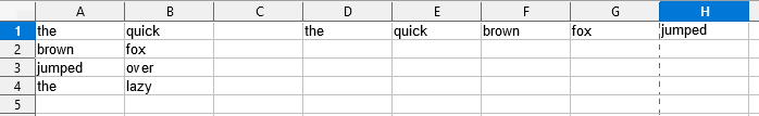
Basically my row should look like this : =A1|=B1|=A2|=B2|= A3|=B3|=A4|=B4

This will be need to be scaled. I have only these two columns, but many many rows. Effectively, I would love to choose the start and end point within these two columns, and the selection will then be split up across the row (see image).

Cheers

I want to transpose them to one long column.

Your title would summarize to I want to transpose them to one long row

Yep, that was a typo. Cheers

You still haven’t made your question clear and accurate. You describe your data “2 columns 4 rows” (which would be A1:B4), but then, describing how the resulting row should look like, write about A1:C(D…)2 - which also raises questions about if the “A1, A2, B1, B2, C1, C2 etc” was actually what you wanted to tell, or a typo again.

And writing about scaling, you don’t describe how the data is scaled. Is the original data growing down (adding rows)? or to the right (adding columns)?

Basically my row should look like this : A1, A2, B1, B2, C1, C2 etc

But you have only 2 columns with 4 rows - so I assume you want your row look like:

=A1|=B1|=A2|=B2|=A3|=B3|=A4|=B4 – or –
=A1|=A2|=A3|=A4|=B1|=B2|=B3|=B4

Apologies, and thank you for taking the time to help. Sometimes it’s hard trying to get the wording right! I did make typos, but hopefully these are corrected now. Thanks again!

If you want your example to start in D1 use: =OFFSET($A$1;INT((COLUMN()-4)/2);MOD((COLUMN()-4);2);1;1)
and drag 7 more cells to the right, but this works for 2 columns only and you have been talking about scaling, which is still not clarified.

Amazing. Thank you. That was what I needed. As far as scaling, I mean only that I will be adding a heap more rows but those two columns will only ever be two columns.

Would you have a moment to explain how that formula works? If my two columns do not start at A1 and B1, but at say E1 and F1, how might I adjust this formula?

Hello,

regarding your last comment and the scaling information:

  • Use formula =OFFSET($A$1;INT((COLUMN()-4)/2);MOD((COLUMN()-4);2);1;1) if you start in D1
  • The formula works for more than 4 rows (but please notice that LibreOffice supports 1024 columns only).
  • The formula does only work for exactly two columns

How does it work:

  • Function OFFSET() requires a reference cell, which is the first parameter (in this case cell $A$1), which doesn’t change
  • Second parameter of OFFSET() requires how many rows to move down (with respect to reference cell A1: Due to the fact that we have two columns to take into account, we need a series of values 0,0,1,1,2,2,3,3 which can be created by =INT((COLUMN()-4)/2) where:
    • 4 is reflecting the fact that formula starts in column D (which is the 4th column)
    • 2 is reflecting the fact that we deal with two columns
  • Third parameter of OFFSET() requires how many rows to move right and for that we need a series of values 0,1,0,1,0,1,0,1, which will be created by =MOD((COLUMN()-4);2) where:
    • 4 is reflecting the fact that formula starts in column D (which is the 4th column)
    • 2 is reflecting the fact that we deal with two(2) columns
  • Fourth and fifth parameter are simply 1;1 since we only, want to reference a single cell (these parameter could be omitted in this case).

See also the formula breakdown in the following file: 2-columns-4-rows-1-row-8-columns.ods

Regarding your question about the start column of your data E1:F1: It should be clear form the breakdown above that it doesn’t matter were your data start (besides the fact that you need to replace =OFFSET($A$1;... by OFFSET($E$1;...). The important thing is the number of the column where you start the formula. In the case above formula starts at column D (column number = 4), thus you have in all parts of the formula a COLUMN()-4. Now, if you start your formula in column S, which has internal number 19, you need to replace COLUMN()-4 by COLUMN()-19 in all parts of the formula.

Hope that helps.

If the answer helped to solve your problem, please click the check mark (:heavy_check_mark:) next to the answer.

I’m so grateful for you taking the time out of your day to help and explain so well.

Just thinking about this some more. As I move down my columns, I copy the formula to the relevant place. Is something like this possible?

=OFFSET($A$ROW();INT((COLUMN()-4)/2);MOD((COLUMN()-4);2);1;1)

It doesn’t appear to be working…

Creating a reference using a formula like in your $A$ROW() never works - you’d need to use INDIRECT().


$A$1 is where your data start but ROW() will yield where your formula is inserted. Thus if you would use that, you’d introduce a restriction, which would read: Formulas need to be in the same row where your data start and you would evaluate ROW() unneccessarily each time you use the formula, just to get the ever same reference cell. If you want stick with that restriction you could use:
=OFFSET(INDIRECT("$A$" & ROW());INT((COLUMN()-4)/2);MOD((COLUMN()-4);2);1;1) , but I cannot see any benefit for that.

More interesting could be the following idea: Define a never changing cell - lets say C1, where you enter your start cell as text.The content of C1 should be$A$1 (as text). Now you could use: =OFFSET(INDIRECT($C$1);INT((COLUMN()-4)/2);MOD((COLUMN()-4);2);1;1) and whenever you change the starting cell of your data, you just change the content of C1.

Cheers. It all working great. I can’t seem to format any cell that contains a number when this formula is used. I’m trying to add quotes around any cell that has a number (after the formula runs). If it’s text, I can apply cell formatting and get the quotes. But if the data is a number, I’m having issues…