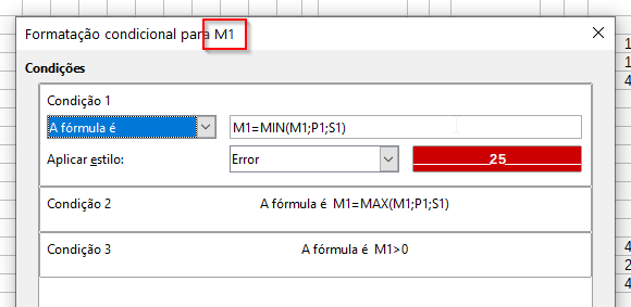
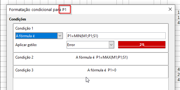
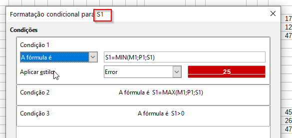
I have three columns (M, P, and S), and I want the values in each row’s cells to have conditional formatting so that the lowest value in that row is my “Red” style, the median value in that row is my “Yellow” style, and the maximum value in that row is my “Green” style. I want the conditional formatting for each row, not each column.
So far, I can only figure out how to do this one row at a time. In Format > Conditional > Manage… there are currently 10 separate conditional formats - one for each row. When I insert a new row at the bottom, the new row’s conditional formatting references are to the previous row number. (“Expand references” is enabled in Preferences.) I have to delete the new row’s conditional formatting, and enter new conditional formatting for that row.
Is there a way to create one conditional format for the three column ranges (currently M6:M16, P6:P16, and S6:S16), so that IN EACH ROW, the minimum is Red, the median is Yellow, and the Maximum is Green? AND… when I insert row 17, the conditional formatting will carry over, and its cells will be minimum Red, median Yellow, and maximum Green FOR ROW 17? Thanks.