Conditional format not applying to "Criteria column"

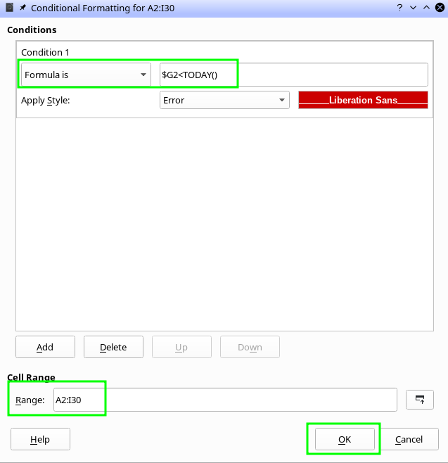
I am applying a formula to a date column:

($G$2:G$30) < Today()

over range
A2:I30

The condition is applying to all the cells in the row that satisfy the condition (A,B,C,D,E,F,H,I), but not the G column.

How do I include the format change on the G column?

($G$2:G$G$30) < Today

Please provide a sample file, since this is not a valid condition (....G$G$30 is one G too much) and Today should be what? (perhaps you mean TODAY()) and to be honest I even would not understand what you’d expect by ($G$2:$G$30) < TODAY()

Edited the double G typing error. The mistake was the ($G$2:$G$30) < TODAY().
This comment cleared my understanding of how to specify the condition, thank you.
“You only specify the condition for the upper left corner cell of your range and the rest is done by the conditional format algorithm when checking all cells of the Cell Range”

Hello,

if your goal in fact is to conditional format the row whose date column G contains a date less than TODAY() then you need to:

  • Select range A2:I30
  • Format -> Conditional -> Condition
  • Condition 1
    Formula is: $G2 < TODAY()
    Apply Style Select your desired style
    Cell Range A2:I30
  • Click OK

Please see the following sample file: ConditionalBasedOnDateColumn.ods

Note Using $G2 in the formula assures that row is being adapted (relative addressing), if condition is applied to the rows of the range and column sticks with G (absolute addressing) while condition being evaluated to columns of a row. In other words: You only specify the condition for the upper left corner cell of your range and the rest is done by the conditional format algorithm when checking all cells of the Cell Range

Hope that helps.