Time format fails on conditional formatting

[InspectorBrain]

So I have a spreadsheet where each line represents a day of the week. I’d like to highlight the weekends. How do I do that?

I opted for a conditional formatting formula and that works. However now I get the following problem: One column of mine has a time format. The cells in this column that are on the weekend (where the conditional formatting formula applies) do not format correctly any more but show a decimal number. I tried different styles and it didn’t change anything.

Time format fail:

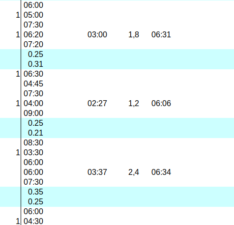
(edit: activated screenshot)

[anon73440385]

Can’t download your file - please upload to this site using **edit** and the clip symbol to attach a file.

[mikekaganski]

When you apply a style using conditional formatting, the cell is naturally formatted using that style. I bet that the style you are applying does not use a time format. Hence when it applies to the cells previously formatted as times, they look like numbers.

[InspectorBrain]

I updated the file.

Correct, the conditional formatting formula does not use the time format: OR(WEEKDAY(OFFSET($A$2;ROW()-2;0);2)=6;WEEKDAY(OFFSET($A$2;ROW()-2;0);2)=7)

How can I combine highlighting for the weekend and a time format

[anon73440385]

Correct, the conditional formatting formula does not use the time format:

It is not the formula causing the problem, but the style applied (formatting the cyan background) - and in that sense a screenshot is not sufficient to provide a sound solution example for you.

You need to split your cell ranges of the conditional formatting and apply a time formatted style (using the same condition) to the column which should show times.

Example: Assuming you have now range A1:G100 using your formula and cell style BGCyan and times are in column C then you need to use the following Conditional Formatting.

Conditional formatting 1 (excludes column C)
Range 1: A1:B100,D1:G100 using your formula and apply style: BGCyan

Conditional formatting 2 (completely new rule)
Range 2: C1:C100 using your formula and apply style: BGCyanWithTimeFormat

[InspectorBrain]

This works, AWESOME!!! Was not aware of the style formatting.
Want to post this as an answer?!

[InspectorBrain]

Providing the answer to the question that Opaque gave:

It is not the formula causing the
problem, but the style applied
(formatting the cyan background) - and
in that sense a screenshot is not
sufficient to provide a sound solution
example for you.

You need to split your cell ranges of
the conditional formatting and apply a
time formatted style (using the same
condition) to the column which should
show times.

Example: Assuming you have now range
A1:G100 using your formula and cell
style BGCyan and times are in column C
then you need to use the following
Conditional Formatting.

Conditional formatting 1 (excludes
column C) Range 1: A1:B100,D1:G100
using your formula and apply style:
BGCyan

Conditional formatting 2 (completely
new rule) Range 2: C1:C100 using your
formula and apply style:
BGCyanWithTimeFormat