How to use pivot table with text data?

[MarcoBrueck]

Hi!

I want to convert the following data (example)

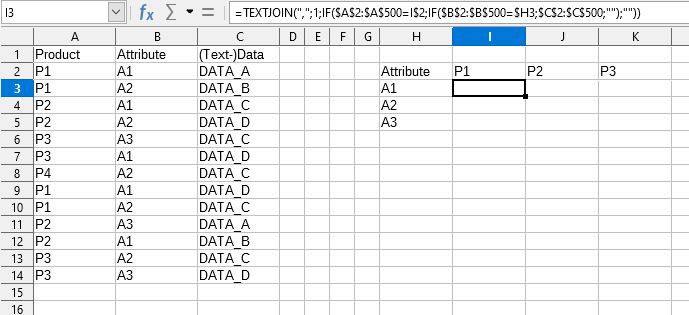
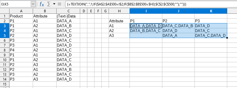
Product;Attribute;(Text-)Data

P1; A1; DATA_A

P1; A2; DATA_B

P2; A1; DATA_C

P2; A2; DATA_D

to a Pivot-table
(Pivot-function);Product;

Attribute;P1;P2

A1;DATA_A;DATA_C

A2;DATA_B;DATA_C

but how?

The Pivot table offers (number) functions like “MIN” which do not work with text data.

a) I would be happy if could use “min” / “max” with text data as well.
b) since - in my case - there is only one data set per field, another function like “first data encountered” could be also useful. But it has to work with “text”.

What can be done?

Best regards

Marco

[JohnSUN]

Yes, you are right, it is impossible to do this using the PivotTable, this tool is intended for other tasks.

You can do this in the following steps.

Get unique values ​​for Attribute and Product - these will be the column and row headers. This is not complicated. Highlight one column in the table and choose Data - More Filters - Standard Filter

Now cut out the unique Product names (Ctrl+X) and make the column headings out of them with Ctrl+Shift+V

I got it like this

For such data placement, the rest of the work will be done by the formula

{=TEXTJOIN(",";1;IF($A$2:$A$500=I$2;IF($B$2:$B$500=$H3;$C$2:$C$500;"");""))}

(This is an array formula, complete it by pressing Ctrl+Shift+Enter)

Now copy the cell with this formula and paste it into the whole table