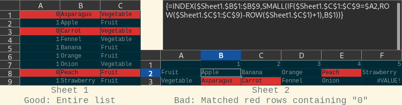
Working on Sheet2, I can use the following formula to look up the "Sheet2.B1"th match in Sheet1, column B corresponding to Sheet1, column C:
{=INDEX($Sheet1.$B$1:$B$9,SMALL(IF($Sheet1.$C$1:$C$9=$A2,ROW($Sheet1.$C$1:$C$9)-ROW($Sheet1.$C$1)+1),B$1))}
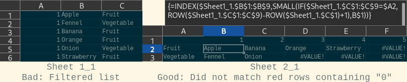
I’d like to exclude rows from the lookup conditioned on the corresponding values in Sheet1, column A. For example, IF $Sheet1.$A$1:$A$9=0 THEN *exclude from row array*. I can achieve this by using Data > More Filters > Standard Filter…, copying the filtered rows to a new sheet, and using the formula above on it. However, I’d like to manage without duplicating any data.
Thanks in advance.
Edit: For example, I’d like to achieve the result in Sheet2_1 without having to filter and copy the data in Sheet1 to Sheet1_1.