
what I’m working with
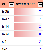
I have a bunch of data columns and am looking to apply conditional formatting to them, color scale or data bar to be precise. I’ve got this part working already and it looks like this:

what I’m lacking
However, not all values in a column should be part of the conditional format. To simplify, whether a value should get formatted and how depends on the type of record (=row) it belongs too. If it’s ID stars with “b” it should use one kind of formatting. But if it starts with “m” instead, use another kind of formatting. Yet if it starts with “s”, use no formatting at all. And so forth:
Currently I have manually defined which rows get which formatting but I have readjust these manually defined ranges for the conditional formatting every time my data set changes (grows, shrinks, etc.). Ideally I want it all to happen automatically.
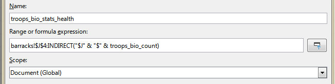
Using the name manager, I have already defined names that describe the relevant ranges and they automatically update when I insert or delete new records, e.g. like this:
my question
But how do I refer to these names (e.g. ‘troops_bio_stats_health’) in the Cell Range field (circled in yellow) of the Conditional Formatting dialog? It only seems to accept literal cell ranges, not names or formulas:

Is is not possible to use names/functions here or am I missing yet a different way to achieve this?