Change style of cell range if

Alexander_13 · January 30, 2021, 5:35pm

I need to apply specific formatting to rows from A1 to Dn if B1:Bn has specific text.

I.e., if B1 has “Send” then change the background at A1:D1; if B2 has “Send” then change the background at A2:D2.

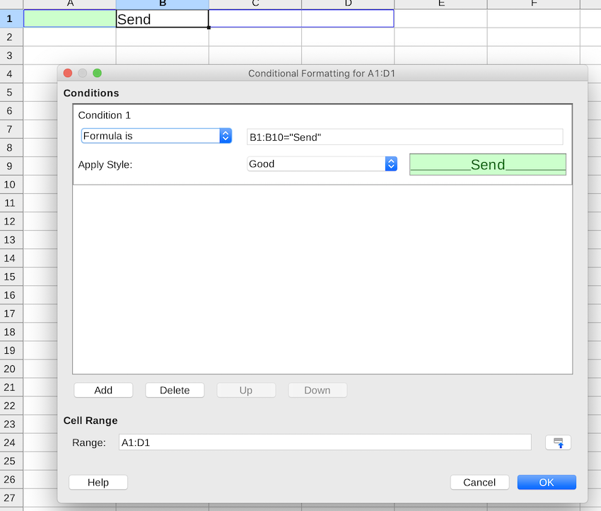
I try this with Format-Conditional; but for some reason, the style applies only to A1, not to A1:D1 as specified.
Besides, it is not logical to create formatting for each new segment (A2:D2,A3:D3,…).
Please advise how to solve this task.

anon73440385 · January 30, 2021, 5:57pm

Hello,

you need to use:
Formula is: $B1="Send" and apply that to Cell Range A1:D<max_numbers of rows> (e.g A1:D999)

see following sample file: Q290462-CF.ods

Imagine the algorithm working the following:

First cell of range: A1
Check formula which is $B1="Send" and perform formatting
Select next cell B1 and adapt formula just like it would do on copy, hence check again $B1="Send" (absolute addressing in columns and relative addressing in row)
and so on for all cells in row 1
Now go to first cell in row 2: A1
Adapt formula just like it would do on copy: hence formula being checked turns to $B2="Send" (row changes due to the relative addressing of row)
… proceed until last row

In other words:

Define the condition/formula for the upper left corner cell of your cell range (here A1:D<max_numbers of rows> ) and assure that the formula is adapted correctly (by the algorithm) by using absolute and relative addressing accordingly.