
I’m having trouble with the VLOOKUP field, which looks into another VLOOKUP field.
In below image, I have the Bestelnummer, which can be looked up via a drop down menu. The ordernumber is 2017BE00001.
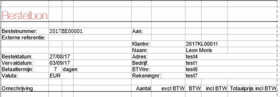
The field Naam searches for this criteria and gives the corresponding name.
As you can see, the name Leverancier / Klant Leon Moris is correctly matched to 2017BE00001
In Image 3, I have entered data in the fields it finds a correct match. As you can see, they are scattered across the field and not in the same line as customer Leon Moris.
My problem is, is that if I remove the VLOOKUP field which looks for the name in Image 2, and type it in regularly, it will find all the correct fields.
This is my code in the bestelbon Naam field:=VLOOKUP(B12;$Inkoopboek.A11:$Inkoopboek.T1000;5)
This is my code in the adres field:=VLOOKUP(G15;$Klantendatabase.A12:$Klantendatabase.I22;4)
In each image, the first field is always the A field
In Bestelbon the row = 10,
In Bestelbondatabase the row = 11,
In Customerdatabase the row = 12
What is causing this behavior?
(edit: activated screenshots)