Filter out items in a column, then count words in the next column

[Carlyle]

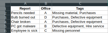
I have a table where I register chronologically reports sent from various offices. The first column contains the report, the second column indicates the office it was sent from, and the third column contains comma separated words that act as tags. The table looks like this:

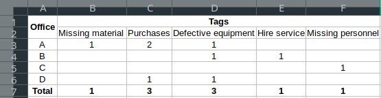
Now I need to get the statistics of tags in total and per office. This means I need to make another table where I re-tabulate the data this way:

I found this formula that gets half of the job done by giving me the total times a certain string appears in a column:

=COUNTIF($Log.C2:C100,"*Purchases*")

This would return the number 3, since “Purchases” appears a total of 3 times in column C of the “Log” sheet. But I have no idea of how to make it filter out the office in column B and then give me only the number of times “Purchases” appears in that office; for example, return the number 2 if I want to get the results for Office A. How can I do this?

[JohnSUN]

Write in cell B3 formula

=COUNTIFS(Log.$B$2:$B$100;$A3;Log.$C$2:$C$100;"*"&B$2&"*")

and drag it to the entire table

[Carlyle]

Thank you!