Can't highlight MAX value in a row, MIN value works...what am I doing wrong??

[jackichad]

Hello,

I am trying to use conditional formatting to highlight the biggest and smallest values in a column. I have setup my conditional formatting to look like the following:

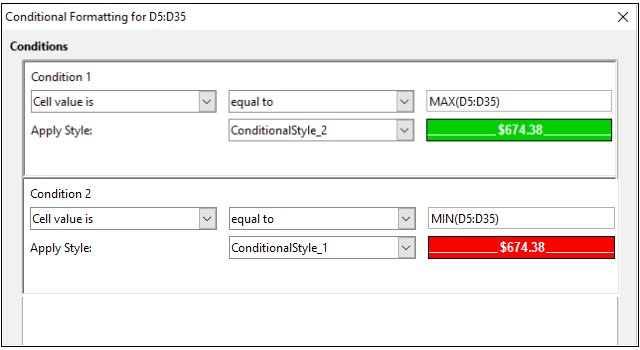
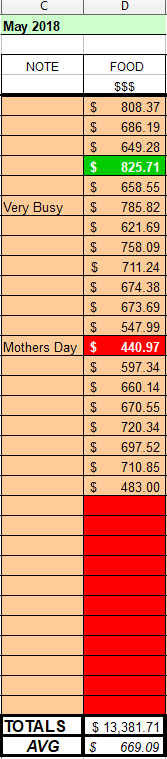
I want to highlight the biggest number in Green and the smallest number in Red. No matter what I seem to do the MAX formula conditional format never works. The smallest value gets highlighted in red, but I never see anything in Green.

Do I need to do something different when using two conditional formats in the same column? This seems like it should be a simple process but I have really been struggling.

Any help would be greatly appreciated. I’m also attaching the first row of my spreadsheet so someone can see what I’m trying to do.

Thank you,
-Chad

May 2018 Test sample.xlsx

[Grantler]

Working on an XLSX file with LO is a dubious idea. Nevertheless you should use absolute addresses for your Conditional Formatting.

Example:

MAX($D$5:$D$35)

After changing the formula worked as it should do. Either as an ODS or as an XLSX file. (LO 6.0.4.2 on LinuxMint)

[Regina]

The formula in the condition has a Basis-cell, in your case D5. That means, that the formula is written as if it is used for cell D5. So for D5 the condition is evaluated as

if ( D5 equal to MAX(D5:D35) )
    apply ConditionalStyle_1
else if (D5 equal to MIN(D5:D35)
            apply ConditionalStyle_2

The cell e.g. D14 is nine rows down, so the entire comparison is shifted down and the evaluation is now

if ( D14 equal to MAX(D14:D44) )
    apply ConditionalStyle_1
else if (D14 equal to MIN(D14:D44)
            apply ConditionalStyle_2

So if you want, that the range keeps the same for all comparisons, then you need absolute addressing in the range.
Try is with Cell value is equal to MAX(D$5:D$35).

But the question remains, why there is not any green. With the formula MAX(D5:D35) there should be green in 825.71 , 785.82 , 758.09 , 720.34 , 710.85 and 483.00. I don’t know the reason. If you copy the range and paste it to a different place in the sheet, you get the green items. A hard recalculate does not force the green items in the original range D5:D24.

Edit: I found the reason. Below the orange range, there is the total in D36. So because of the shifting from D6 downwards, the range, which is used for comparison always contains the total. Therefore no cell of the orange range can be the maximum.

[kompilainenn]

You may use:

for first Condition : Cell value is - top 10 elements - 1

for second condition: Cell value is - bottom 10 elements - 1

ps: number 10 is a mistake in GUI. Need enter value in to right field

[mikekaganski]

This is a better alternative to say “min/max value in the given range” instead of hardcoding the range in the formula.

[jackichad]

This is a great start! Just two quick questions:

1. Once I add the formatting to my range, I get my green(high) and red(low) but it also marks all empty/blank cells red, which makes sense since they are all a small value. Is there a way I can make it ignore blank cells until I input a value into it?

2. Once I get this working, will it be simple to copy the formatting to other columns?

Thank you very much!!

[kompilainenn]

1. There is a way: create else one condition for your range (push Add) with Cell value is - equal - “” with style Default, and move it to top of list (push button Up)
2. Yes, you can set a new size of range