
I want to copy conditional formatting rule from 1 cell to another and have new conditions for the new cell that I can update based on the original rules without making the condition a range. I am looking at 1240 new conditions to create unless there is a way to do this. Please, any insight would be greatly appreciated.
Individual cells for weekdays need to change color based on individual selections by day which are in another set of cells.
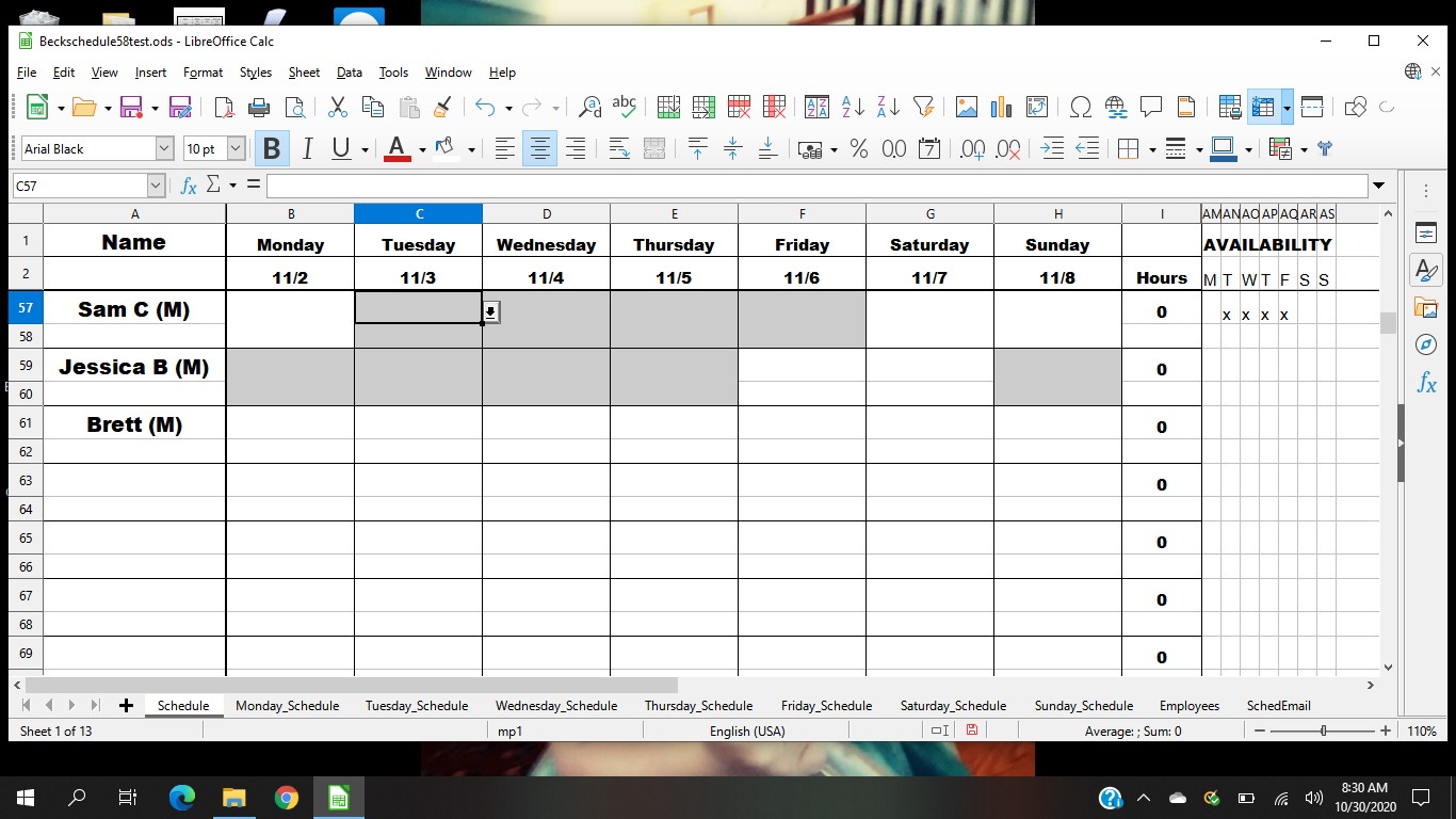
see attached
Hi,
could you give a more detailed example of what exactly you want to do.
preferable with Before and After display.
PS:
You can edit/attach screenshots and documents to your question.
Later.
Thanks. Please see added screen shots
I am 99% sure, that i misunderstood your requirements.
It looks to me like you are trying to apply two conditional formats to (each) cell.
And you want to be able to copy the 1st conditional format as is and change the
second condition when you apply it to another cell?
Couldn’t you apply the first conditional format onto all cells?
And for the 2nd conditonal format, i dont quite get the conditions,
how you want it to change.
Maybe you can attach a document (snipped) with a couple of cells manually filled out.
Later.
Actually, I want 2 conditions applied. 2 to b57 and the same to b58. This changes the color based on the value in am57. I then want to copy b57 formatting to c57, b58 to c58, and change the formula in those to check the value of am58. And continue to do this for the rest of the weekday cells.
Sorry, the c57 and c58 formulas should reference an57
I think this would entail the ability to copy conditions on the conditional formatting management screen.
Just not sure if there is a way to do that without adding each individual rule by cell.
Mmmh,
there is a similar older request, which states that the conditional formating can be copied
Yes I saw that, but when I copy and paste just the formatting, it doesn’t creat a new rule for the new cell, it just makes the old condition a range from the old cell to the new cell. I then cannot change the formula because doing so would invalidate the availability status by day as reflected in the x’s in am57-aq57.
-1- Do you feel sure the basic design of your sheet(s) is well considered?
-2- What’s the reason for what you think to need so many (slightly) different CF settings?
-3- Might it be you are asking a question concerning somethig you would need to continue the way you started, while a somehow changed approach would make everything much easier?
There is something called “X-Y paradox” (way/goal") now and then. If you describe what you finally want to achivee, an experienced user might suggest a different simpler and more efficient way. Achieving the overall goal can be much simpler than to do the next step on a doubtable way.
Hallo,
What you need are two conditional formats.
- Mark
B57:H57→ Formula is:AM57 = "x"→Apply Style: gray→ Ok. - Mark
B58:H58→ Formula is:AM57 = "x"→Apply Style: gray→ OK.
Then copy B57:H58 and paste that at B59, B61, B63 etc.
My operating system: Windows 10 Home (x64)
My LibreOffice versions: 6.4.7.2 (x64); 7.0.1.2 Portable
If the questioner wants exactly what @PKG found out, the actual problem is to get conditionally formatted cells of two consecutive rows based on conditions only entered into one of these rows.
Since the questioner also told us he was afraid of needing to define 1200 CF, I would assume there are up to(?) about(?) 600 Jessicas and Bretts. Doing it the way suggested here this would require to list 300 ranges for each of the two CF definitions. In addition the overall CF range needs to be filled by pairs then what may be error-prone.
Try the alternative solution from the file attached below:
ask274147FormatConditionallyTwoConsecutiveRowsBasedOnConditionOnlyPresentInOneOfThem.ods.

Thanks for your suggestions. I’ve tried everything I can think of and determine that it’s not possible to do what I want. I need to change the formula in each cells conditional formatting to reference the correct column in am-as. If I enter a stand alone conditional formatting in c57,for example which it lets me do, to accomplish this, it does not work. The problem is the need to change the formula by cell. Anytime I try copying it makes the conditional format a range, which I don’t want. Thanks again.
SOLVED. PLEASE SEE MY COMMENT TO NEWBIE-02
Did yo consider at all a CF using te ISODD(ROW()) part - or a similar construct?
That’s the appropriate way to make CF for pairs of rows.
I demonstrated it in the attachment to my comment on the answer by @PKG.
Might you tell in a clear way for what reason “The problem is the need to change the formula by cell.”
What kind of changes are needed “by cell”?
If the change is just the adaption of the column reference, this is automatically done by relative addressing (what you used anyway in the posted formula). The colums for your “x” markers (AM through AS) are - and must be - consecutive in the same way as the cells you want to apply CF to. Where’s the problem if not to make the single “x” work for two rows?
hello @Alsans3,
a ‘kiss’ try - try to learn working with ‘not completely perfect’ tools with simple workarounds …
take one formatted cell you have,
copy to another sheet with ‘ctrl-c’ - ‘ctrl-v’,
change something in the format definition there,
copy back to first sheet,
you now have two independent format definitions there which you can edit and apply to ranges …
ok?
P.S. ‘solved marks’ and ‘likes’ welcome,
click the grey circled hook - ✓ - top left to the answer to turn it green if the problem is solved,
click the “^” above it if you ‘like’ the answer,
“v” if you don’t,
do not! use ‘answer’ to add info to your question, either edit the question or add a comment,
‘answer’ only if you found a solution yourself …
P.S. II @Zizi64, that bug is ‘nice’, but imho irrelevant for this question, bug a malfunction when moving cells with conditional format, question about possibility to copy and edit conditional formatting
Thank you. I tried what you suggested and when I pasted the individual new cell format back to the original, it still changed the conditional formatting to a range. However, even though looking at the condition, it appeared that it would not work since the formula for the range still showed it referring to am57, it did now work. It did not work before. The colors of the 2 cells at c57 and c58 changed based on the contents of an57. I then used ctlc and Ctlv to copy and paste this to the rest of the columns and they updated properly also. They correctly reflect the contents of am57-as57. I am also able to copy in this manner to all the rows, and they work nicely. I have 90 rows in this spreadsheet. Copying this way is fabulous compared to thinking I had to 1240 manually entered conditions. So thank you again.