Countif based on last character in text string

I have a column of text based codes. Some end with F, some with A and some with - .

A1 KnotsP-A
A2 SaucyF–
A3 B-SweP-F
A4 StancF-F
A5 RoothF-F
A6 GrainF–
A7 RavenP-F
A8 GermaP-A
A9 ParkeF-F
A10 LucieFE-
A11 Top MPEF
A12 WarneF-F

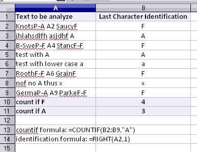
I would like to be able to count how many end with F.
I have tried a number of variations suce as:
=countif(A1:A12,.f)
and
=countif(A1:A12,"
.F")
and
=countif(A1:A12,"=.F")
but they do not work.
=countif(A1:A12,"W.
") works, returns 1

Please note that the formulae include the wildcard asterix but they don’t seem to show up on this blog.

Any help would be great.

Thanks
FB

Yes, regular expressions are enabled. As a result countit based on the first character works for example =countif(A2:A12,“W.*”) returns 1 but countif based on the last character does not.

=countif(A1:A12,".*F")

Have you enable regular expression?: Menu/Tools/Options/Calc/Calculate/ Enable regular expressions in formulas.

I can confirm that this formula works fine with regular expressions enabled. Of course, it will fail if the strings have trailing spaces after the last “F”.

the joys with regular expressions is that you can also make it “F followed by optional space” if needed :slight_smile:

Pinging @jorendc: Could you please lend your mac-testing skills to this question? Please let us know if mariosv’s Answer seems to work. If it acts differently on different OSes, then this question gets a free trip to you-know-where! (no, not Mordor… although it’s about as scary to some users :wink:

You could always create a new column which has only the last character, e.g with this formula: =UPPER(RIGHT(TRIM(A1);1))

TRIM() removes leading and trailing whitespace, RIGHT() picks given number of last characters and UPPER() converts everything to UPPERCASE.

How to count certain characters? =COUNTIF(B1:B9;"F")

@mahfiaz: this is a nice solution! It differentiate upper and lower case characters as well as spaces. Well thought through!

Hello

Thanks but that gives a result of 0.

FB

Please don’t use the answer functionality for comments.

I have double checked for blank spaces following the last character and also manually entered a sample list on a new sheet and still it returns 0. The same problem exists when I try it with Open Office. I am running OSX Snow Leopard on an iMac.

Ok, so we need someone who could test this on a Mac. I’ve only Linux an Windows available, sorry.

Thanks, I have also tried a workaround using SUMPRODUCT and REPLACE but still get 0.

Would any one have a suggestion on a SUMPRODUCT & REPLACE formula that might work? Or a different work around?

Could this be a possibility: Use right(cell, lenght(cell)-1) to identify the most right character and then work with countif?

I just had a couple of minutes and could make a test. This is the result according to my understanding of the question.

Should this be wrong, I need more information on the task.

image description