IF + VLOOKUP displays result as "true" but not the value

[salary_man73]

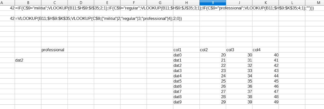
Using the following formula to return a value based on criteria for a wargaming army sheet I’m making:

=IF(C$9=“militia”,VLOOKUP(B11,$H$9:$I$35,2,1),IF(C$9=“regular”,VLOOKUP(B11,$H$9:$J$35,3,1),IF(C$9=“professional”,VLOOKUP(B11,$H$9:$K$35,4,1),"")))

Where C9 is the grade of the unit input by the user (“militia”,“regular”,“professional”).
Where B11 is the type of unit input by the user corresponding to units in the table array (e.g. “HMG”).
Where H9:I35 is the lookup array of the various units and points costs.
Where my lookup array IS sorted alphabetically A-Z.

The formula will display “TRUE” in the cell and a “=sum()” below it will display the correct sum of multiple cells. I want the if+vlookup formula to display the number value it is looking up in the associated array.

Example:

HMG TRUE

HMG TRUE

Total 20

What exactly am I doing wrong? I’m fairly confident this would work in excel.

[plp]

just format the cells to number

[mariosv]

Maybe with a more simplified formula, using an inner array, you don’t need the IF, and easier to add more values.

=VLOOKUP(B11;$H$9:$K$35;VLOOKUP(C$9;{"militia"|2;"regular"|3;"professional"|4};2;0))

I think it was a format bug some time ago, not with the value, in BOOLEAN format all positive values are showed as TRUE, please what is your version?