COUNTIFS - How to match partial string

Yes, attached to original now. Sorry; I did not see how to upload anything at first.

Also, when you open it, please note, on Sheet “QQQ 3-5D”, cell H7, both it’s formula and it’s comment. For some reason that seems to be counting wrong (that sheet, and also “SPY 3-5D” & “MES 3-5D”). You can note that I have added zeros to cells like J15, J23, J37, J40, because if they are blank, it does not count them as zero.

I see two problems:

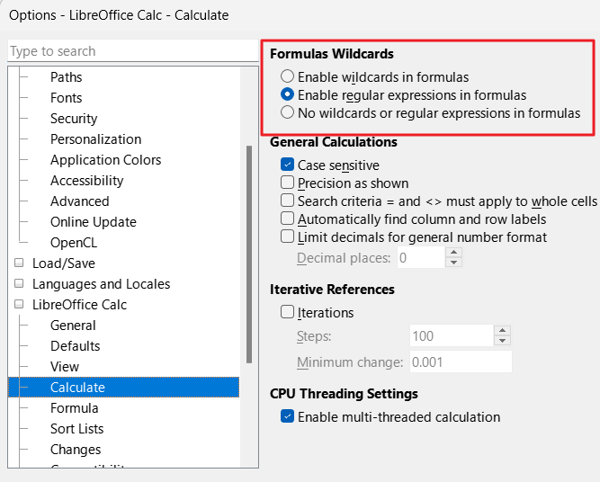
  1. You have not defined any label. Defining labels is in menu Sheet > Named Ranges and Expressions > Labels… If you do not define labels yourself you need to enable option “Automatically find column and row labels” in Tools > Options > Calc > Calculate. But the latter will sometimes fail depending on the structure in your sheet.

  2. Labels have to be enclosed with straight Apostrophs. So not Date but 'Date'.

Thank you; response much appreciated.

  1. I had wondered if there was something like this. Very good info to know.

  2. Interesting… because that is not how it is in the sample file (attached).
    The only mods of interest I saw in the sample is that underscores are used in place of spaces in the labels.

Are settings (like my disabling of “Search criteria = and <> must apply to whole cells”) document-specific, or go across all docs? I would presume the latter, but I’m sure it makes more sense for some to be specific.

Also, did you see any reason for the ‘bug’ in my cell H7 of “QQQ 3-5D” sheet; why I had to subtract one to make it accurate?

functions_ifs.ods (19.9 KB)

Cell: J71

J71. Yes, thanks, I see; another Monday holiday, where I need to make it zero, like J15.
The formula uses <>

=COUNTIFS(A9:A140,"Monday",J9:J140,"<>0")

Yet I thought a blank cell was supposed to count as zero. Is there a way to make it treat empty cells as zero, so I do not need to set J15 & J71 to zero?

You could search with regular expression.
=COUNTIFS(A9:A140,"Monday",J9:J140,"[1-9]").

Regular expressions must be permitted in formulas for this purpose.
Tools → Options → LibreOffice Calc → Calculate ►

1 Like

… or without changing the options:
=COUNTIFS(A9:A140;"Monday";J9:J140;"<0") + COUNTIFS(A9:A140;"Monday";J9:J140;">0")

No, a cell cannot be >0 and <0 at the same time. :slight_smile:
My formula is an attempt to combat empty cells.

of course …sorry my fault!

1 Like

Or a formula that works independently of the language.

=AGGREGATE(2,6,IF((WEEKDAY($A$9:$A$140,2)=1)*($J$9:$J$140<>0)))

How do you match an empty cell, like replacing the zero:

=COUNTIFS(A9:A140,"Monday",J9:J140,"<>""")

Can you use backslashes?

=COUNTIFS(A9:A140,"Monday",J9:J140,"<>\"\"")

(LeroyG added Preformatted text to the formulas)

=COUNTIFS(A9:A140,"Monday",J9:J140,"<>")

That does not appear to work…

Is comma the correct separator for you? For me it would be a semicolon.

What’s wrong?

You are right; the help does show semicolons. Apparently it [mostly?] works with commas too. I will try it with “<>”…

I tried to change my commas to semicolons, but search and replace wasn’t working and in fact when I just edit a cell (like H7 in QQQ 3-5D), it just changes them back to commas. The odd things is, it works fine with the commas, but then changes from the 7 it should be to 30 because of all the Mondays in column J that have zeroes.

Because column J has this formula:
=IF(I53<=0,0,I53-G53)

Now if I go to every “Monday” cell in Col J and hit delete, I get my correct number of 7.

But if I change the formula in Col J to:
=IF(I53<=0,"",I53-G53)

then each unused cell does indeed show blank, but I still have a count of 30.

Is that because when it looks for nothing, “<>”, it is actually matching the formula of the cell, and so does not count it as blank?

Yes.

Backslashes don’t escape a double quote character, doubling them does, so

=COUNTIFS(A9:A140,"Monday",J9:J140,"<>""""")

but that is not what you are looking for, because it would match only cells not containing a string with two literal " double quote characters.

Whether to use the comma or semicolon function parameter separator depends on the locale you work in; in locales that use comma as decimal separator it can’t be used as parameter separator, but using semicolon works in all locales, hence we use it here for examples, even if afterwards it will be converted to the set parameter separator, e.g. comma.

Any idea why that does not work then? (see second half of previous post)

Okay, I must have misunderstood. You said:

I thought “<>” means ‘not equal to blank’, but you were saying it’s ‘not equal to non-blank’?

Perhaps it would be easier if you can give me the right formula. So I want to match rows that have Monday in the first column AND are NOT blank (in Col J), and thought it was this:

=COUNTIFS(A9:A140,“Monday”,J9:J140,"<>")

Can you correct it for my intent?