format number as currency based on next cell content

Hello,

I have a table with two columns:
Column A = numbers
Column B = currency codes (i.e. USD, JPY, EUR, etc…)

example:
https://drive.google.com/open?id=1tvm1mOgys0AYPkXaCN1xCUzyHu3_Vtil
^ (screenshot)

how can I have cells on column A to automatically format as the correct currency based on the code column B on the same row?

Copy format codes from Format → Cells, Number, Currency into a lookup table.

D         E
~~~~~~~~  ~~~~~~
currency  format
USD       [$$-409]#,##0.00;[RED]-[$$-409]#,##0.00
EUR       #,##0.00 [$€-612];[RED]-#,##0.00 [$€-612]

Now use the TEXT function and look up the format. Enter the following formula for A2.

=TEXT(250000;VLOOKUP(B2;D$2:E$3;2))

The result:

formatted currency values

Thank you Jim, very interesting, I didn’t know about the TEXT function; I’ll give it a try!

Meanwhile, it seems like I have succeeded in using conditional formatting, like this:

https://drive.google.com/open?id=1x0xKtDXeGGmbfvj_U629zQ8D6PNxVIbk

(to see the conditions applied to the data in your screenshot, replace Q52 and R52 with A2:A500 and B2 respectively … I had to create a custom style for each currency I am testing against)

It took me a long while to figure it out, because I was missing to first clear all existing formatting for the cells in column Q (column with numbers in my table)

The table I am building is a work-in-progress, I haven’t had the chance to 100% verify this approach, but at first glance it seems to work.

This is a good solution as well. I upvoted so that you have 20 karma points, which is enough to accept your own answer if that’s what you decide.

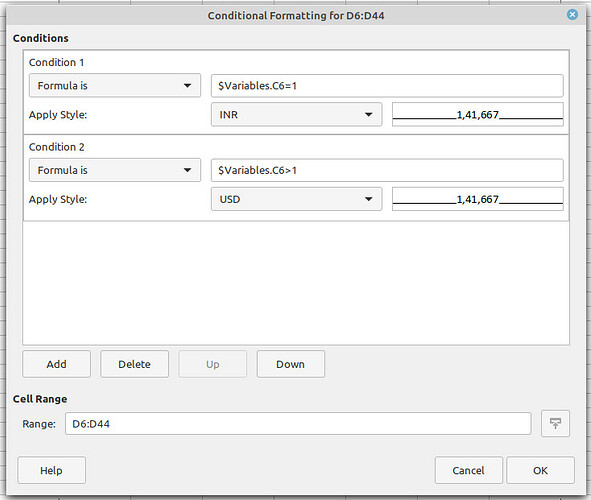
this is what I did and it’s working for me:

  1. created two styles namely USD and INR
  2. created a conditional format for the range I needed with 2 conditions:
    2.1 condition 1 was Formula Is > referenced the cell here with the value it needed to look (=) for and applied the appropriate Style
    2.2 condition 2 was Formula Is > referenced the same cell as above with any other value (>) other than the one above and applied the appropriate Style

So now I just apply this conditional format to all cells that contain currency values and based on the C6 value in sheet $Variables the correct currency symbols are displayed.

hope this helps