But they don’t provide the targeted subtotal count on a filtered array which is what I’m trying to achieve.
Ignorant is what ignorant does. Would you disagree?
I step through the Formula with next|back-button.
Good to know! I thought it was related to your highlighting of the function component so couldn’t replicate it.
Now all I need do is get it to say “4” - then I’ll have learned two new things.
Just to clearify: OFFSET(A6:A16;……; 1) return 10 different entrys, and the outer SUBTOTAL(3;…) is evaluated 10times
If it’s accumulating all those binary indicators and evaluating everything for the number of rows in the array, that probably implies it would develop indigestion on an array of 3500+ rows - even if I could get it to count instead of sum.
That’s the convincing argument to abandon the approach. My current process just does it once per row and I thought array processing would reduce that volume.
That’s the second thing I’ve learned today.
thats also FALSE, Pivottables “react” on Filter-settings in the Sourcerange, …and provides itself Filter-options on every “corner”, and of course its a matter of ~3Mousclicks to aggregate with COUNT (additionally or instead) SUM
of course, remove the “tail”:
=SUMPRODUCT((SUBTOTAL(3;OFFSET(A6:A16;ROW(A6:A16)-MIN(ROW(A6:A16));;1))))
but at this state the outer SUMPRODUCT(…) is superfluous, and at the End of the Day we come back to simply:
=SUBTOTAL(3;B6:B16)
But with this I can’t say count only the items >72,3 in an array that isn’t already filtered to exclude those <=72,3
Switch from some Filter to →→Standardfilter, set your desired Options and youre done.
The whole point of my exercise is that I don’t want to keep manually changing filters to “exclude” from the display what I don’t want to count.
I want to say "how many records in column L are greater than 73,5 - just tell me the number - Oh, by the way, I’ve now filtered out everything that occurred in February so the new count is automatic. Hmmm, interesting, how many in column N are now at -0,4 and how does that change if I add February back but remove July - and about 3500^5^6 other permutations. All of which I can do with the 5 extra columns of helper cells which monitor the values on a row by row basis and which I was hoping to replace with an array function. What would be perfect would be subtotal(3, IFANDOR(IFANDOR(IFANDOR - with all the factors being cell lookups of such operators as <,<=,=,>=,>, Val(x),Col (L).
I do realise this is an extreme/advanced “single” function but it would be replacing thousands of active cell formulae - if it were possible. I think it’s probably more akin to a user-defined function in Excel’s LAMBDA().
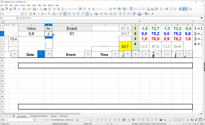
I currently achieve it with three “source” cells using an HLOOKUP() to define which column’s filter SUBTOTAL(x,) will contain the result. It does what it says on the box but I was experimenting to see if it could be “streamlined” with an array function to remove the 15000 helper cells and work directly upon the “real” data cells.
I think the function name is probably MIRACLE().
Did you view the file? Is there a way to get it into ASKLo or do I have to leave the link to my GDrive in perpetuity?
The usecase for SUBTOTAL is about using Filters, if you want to not use Filters at all, or in humptie combinations with other Criteria, you should not use SUBTOTAL, but something of SUMIF[S], COUNTIF[S], SUMPRODUCT.
Sorry I get the Audio-part only, no video!
is it ok to mail it to you direct?
I use the COUNTIF() in my helper cells because they count unconditionally of the filter setting but the SUBTOTAL() at the top of each helper column then only accrues the result if it’s not “hidden” by a filter. Best of both worlds, I can exclude on generalities and include on specifics.
I just downloaded it and allowed it to play directly from the download and also only got the audio. However, using VLC and just reloading, it seems to work
Makes no difference… try to upload as .mp4 instead .mkv
Audio got a bit clipped
Maybe this is more indicative
I can have any combination of active filters on both data entry and subsequent calculations, ADDITIONALLY I can identify a value <,<=,=,>=,> and the appropriate column and it returns the count of those values in the target column that are visible anywhere in that column - currently 3500 rows x 3 columns + the 430 rows of two columns being the two rightmost elements of the framed row.
You are mis-using a spreadssheet as a database. This is one of the biggest misconceptions in computer history. The pivot table feature is a big concession to all the users who struggle with this (the majority I think). It works like a database query. Once you run a query, it returns an entire table from another table and dumps the result to a range of spreadsheet cells. But you have to run that query. I have seen a pivot table on a Calc sheet aggregating millions of database rows in under a minute time. You must not expect that every change of a value re-runs the database query automatically. That could make the whole thing unusable.
RIght-click>Refresh does the trick. or Data>PivotTable>refresh or
ThisComponent.Sheets(0).DataPilotTables.getByIndex(0).refresh()
You may put the pivot on another sheet and run such most simple macro when the sheet is activated.

