calc icon set formula

I’m trying to get the conditional formatting to work with the icon set.

For icon sets that are in the same cell it works nicely

so if I have A1 with a value of 0 and A2 with a value of 1 it will show a traffic light depending on that value.
What I’m trying todo is to have a traffic light in a cell without text in it, so make it dependent on another cell (which I can hide then).

So I have a colum A and in those cells is either 0 , 1 , or something else
In column B I want to have a traffic light depending on the value of the Cell left to it from column A.

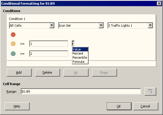
So I go to B1 → conditional formating → Icon set, change Percent into “Formula” and there starts the problem… whatever I try there won’t work so formula “=A1” or “IF(A1>0)” etc… I’m sure I’m doing something stupid… any idea?

  • Type in A1 the values (in my example they are 0, 1 and 2).
  • In B1 imput the formula =A1.
  • For B1 choose menu Format - Cells… - Numbers tab, and in Format code field type a no-break space (Alt+0160¹); this will show an “empty” cell.
  • To set conditional format, choose Format - Conditional - Icon Set….
  • In the yellow light field type 1, and choose Value.
  • In the green light field type 2, and choose Value.
  • OK.

Conditional Formatting - Traffic Lights 1

See sample file.

¹ To obtain the no-break space you can also previously edit a cell, type U+00A0 and inmediatelly press Alt+X, select and copy this space to paste later in Format code.

Made with LibreOffice 6.3.6.2 (x86); OS: Windows 6.1.


Add Answer is reserved for solutions.

Press edit below your question if you want to add more information; also can comment an answer.

Check the mark (Correct answer mark) to the left of the answer that solves your question.