
I have a “legend” on a Calc sheet with 5 different values in 5 cells.
for example:
A1 = 4.9
A2 = 5
A3 = 10
A4 = 15
A5 = 20
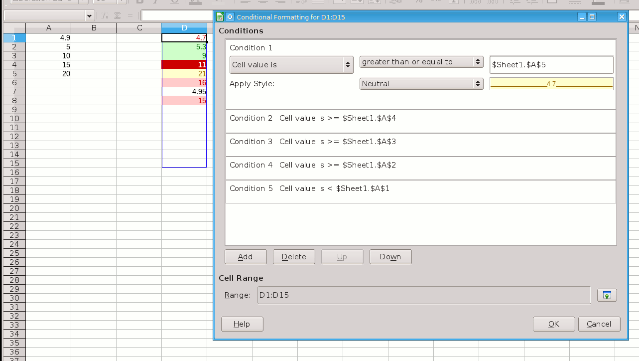
I want to apply conditional formatting to a range as follows (psuedo code):
condition 1: IF <A1
condition 2: IF >=A2 AND <A3
condition 3: IF >=A3 AND <A4
condition 4: IF >=A4 AND <A5
condition 5: IF >=A5
Unfortunately I am getting stuck entering any useful formula in the “formula-is” of each condition in the conditional formatting dialog.
Thanks in advance for any guidance.
 to the left and, karma permitting, upvote it. If this resolves your problem, close the question, that will help other people with the same question.