Conditional gradient style for irrelevant in the condition cells

[halloo]

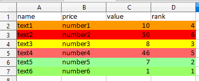
I want to essentially link the style of other cells in the same row to a specific column. So that the entire row is colored the same color.

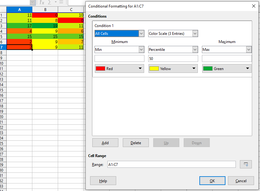
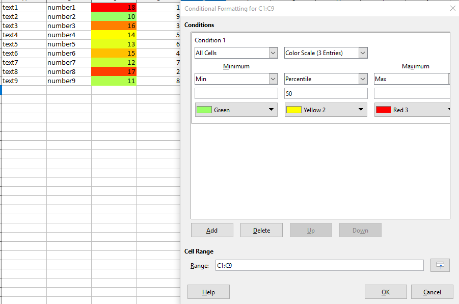
all cells → color scale(3 etnries) applied to:

range: C1:C9

I’m trying to color the rows on the left(text&number) with the same color either by:

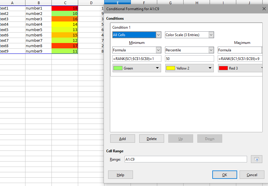
range: A1:C9

=RANK($C1;$C$1:$C$9)=1

=RANK($C1;$C$1:$C$9)=9

OR I’ve tried another way by moving the range() formula into a separate column:

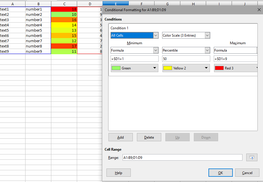
range: A1:B9;D1:D9

=$D1=1

=$D1=9

having just one style, something like:

range: A1:C9

=MIN($C$1:$C$9)

=MAX($C$1:$C$9)

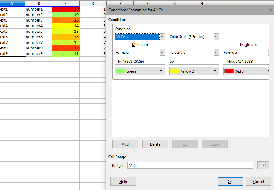
does the same thing in one style, but not the entire rows

[mikekaganski]

But how could it differentiate with e.g. this:

[halloo]

@Mike2 in your example the conditional style just looks at the value of every cell relative to all other values in its cell Range.

But I need is to color the rows the same color, for example:

The only relevant for the coloring style condition column is “rank” (Cell Range = D2:D7), the relations of values in this column represents that gradient color, the values in D2:D7 are calculated with: =RANK(C2;$C$2:$C$7;1) function.
(“rank” column represents color, I’ve added it for simplicity, so ideally I’d want it to just be in a formula somewhere, leaving only color)