Last five oldest dates within past 2 years

Given a column containing dates, how to:

  • conditionally format the last five oldest dates in the past year (24 months)? I would like to then use it is one of two criterias–I suppose whatever is returned can be used in e.g. COUNTIFS.

  • print the value of the oldest date in the past year plus 2 years?

Much appreciated.
untitled.ods

Please edit your question and attach a sample file, explain in it what you want to do.

@mariosv Attached. I made slight tweaks to what I’m looking for since I used a more accurate representation of my data (premise is the same, values of the constraints changed and updated in original post):

  • Looking for formatting rule for all dates highlighted in orange, which are dates that are of “Type P” and are within the past 2 years (24 months).

  • Keep a count of the dates that satisfy this criteria (6 in example).

  • Of these dates that match the criteria, print the oldest date (10/21/18 in example).

  • Print the date of the drop-off of the oldest date (10/21/20, which is 10/21/18 + 24 months).

  • Not asked in the question, but formatting of the cells in the “Fee” column for upcoming fees. Upcoming fees are those that are the 1st of the next month of 1 year plus the respective date date that is within 30 days (90 fee has red font color because its corresponding date is 4/15/19 which means fee is due on 5/1/20 and that is within 30 days of today).

Thank you.

1585927504515277.ods

Is there any particular reason to use absolute reference for rows but not for columns for this specific set of data? I just don’t tend to use absolute references for anything unless it is necessary. Would like to follow good practices.

If only for one formula absolute it’s no needed, but if are going to copy yes, so it’s like a prevision for copy.

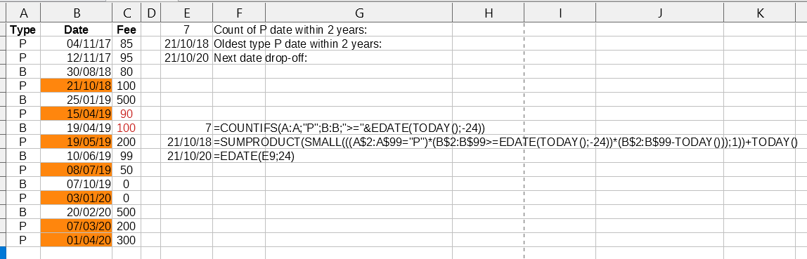
@mariosv Sorry, one more question: how does matrix multiplication work and could you break it down in this example for the formula =SUMPRODUCT(SMALL(((A$2:A$98="P")*(B$2:B$98>=EDATE(TODAY(),-24))*(B$2:B$98-TODAY())),1))+TODAY()? I could only find documentation of it here but I’m not sure how the matrices are generated and how it computes the final result. All I can understand from that formula is (A$2:A$98="P") and (B$2:B$98>=EDATE(TODAY(),-24) as constraints. It actually took my a while to even figure out using AND condition is possible with this trick so I’m really curious how it works so I can make my own.

Also, what is the purpose of B$2:B$99-TODAY() and then the final TODAY() that is added to the SUMPRODUCT?

Much appreciated.

SUMPRODUCT() it’s to force the formula working as an array, instead using [Ctrl+Shift+Enter] to enter it as array, as SMALL() produces a single value there is no problem on using SUMPRODUCT(). Multiply comparision’s results it the same as AND(). The trick if there is any, it is B$2:B$99-TODAY() to get the small value, and sum TODAY() to the result to recover the wanted date.

@mariosv Why is it B$2:B$99-TODAY() and not simply B$2:B$99 (which yields a wrong result that I don’t underrstand) as the third AND() condition for SMALL()? My understanding is that cells that satisfy all the conditions will then be added to an array internally that SMALL() then operates on, so shouldn’t the dates be passed to SMALL() directly? Why subtract TODAY() for every date cell and then add it back after?

Thank you.

Because if not, for SMALL zero values are the small value, in this way we get negative values, being the most negative the small.