
The last entry may not be the last day of the month.
I have already spent hours searching the web for a solution but without success.
Just to try to clarify…
In Worksheet ‘A’ I have my bank transactions with running balances.
I have more than one bank a/c in this worksheet.
All transactions are formatted the same, are in the same columns, and each bank a/c is separated by blank rows.
This is so I can code the transactions and then summarise the codes from all bank a/c’s using one pivot table.
In Worksheet ‘B’ I want to show the last balance of the previous month for a specific bank a/c.
The previous month is formatted as a ‘date’ in this worksheet.
So I need a formula in Worksheet ‘B’ to go to Worksheet ‘A’, then go to the cells containing the transactions for the particular bank a/c I want to use, go to the last row of the last transaction date for that month (which may not be the last day of the month - and there may be multiple transactions on that date), then select the ‘balance’ to show in Worksheet ‘B’.
I don’t use macros.
Perhaps something like a VLOOKUP function combined with something to find the latest transaction in the month?
hi WW,
[2. edit - coloured sheet]
coloured sheet - download here
step by step,
- download sheet,
- see balances pulled from E8, E10, E13, E14 pulled to L4, L5, L7, L8,
- put some of your data in the blue cells, dont touch any other,
- check if it works producing results in L4 … L8,
- insert cells as needed in col. A:F, cells!, not rows, insert with e.g. marking A10:F10 and ‘ctrl +’ and ‘move cells down’, don’t insert in row 4, but between rows 5 and 15, that will automatically adapt all formulas,
- correct the cells in col A, E and F, A - bank names, E - copy from E4, F - ascending integers,
- check if results in col L still correct,
- put more data in,
- if it fails somewhere got back and try to debug,
- you have one working sample, should be possible to work on from that,
- you may change anything to your need once you understood the contruction …
[/2. edit]
[edit - reg. new info]
considering that the workflow you describe fits better for a macro than for formulas although the ‘data structure’ is still difficult, your listed data is not very clear, it is nonsense to nail long boards together at right angles before you carry them through a narrow door, to spill data together when you need them separated for evaluation, to give screws to someone who is used to use a hammer and you might want to use pen and paper instead of calc 
and that, as you use pivot tables? - respect! -, i’m perplexed why you didn’t already solve it with that … ???
i reworked my silly sample, you can download here:
hope that helps, feel free to place the framed range on a separate sheet with [ctrl-x - ctrl-v] and! to check for mistakes! provided ‘as is’ and ‘wow’ - ‘without any warranty’!
reg.
b.
P.S. upload - you need ‘karma’
[/edit]
there will be plenty similar questions with - good - answers in ‘ask’ and the web, just for some exercising i’d construct a little sample for you:
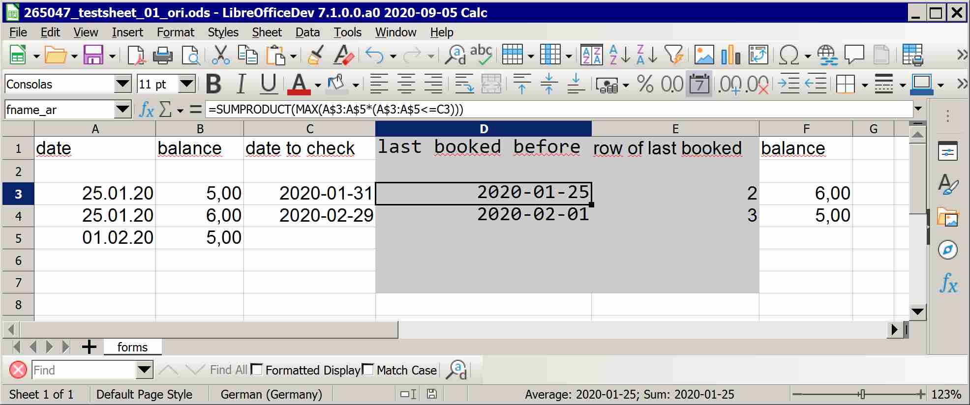
it works with two intermediate columns to avoid too long formulas, of course you can integrate the grey’ed columns into the balance formula,
i’m not! sure if it holds for all cases with two or more identical booking dates … i remember that someone wrote somewhere that there is no guarantie which cell you get in such cases …
P.S. ‘solved marks’ and ‘likes’ welcome,
click the grey circled hook - ✓ - top left to the answer to turn it green if the problem is solved,
click the “^” above it if you ‘like’ the answer,
“v” if you don’t,
do not! use ‘answer’ to add info to your question, either edit the question or add a comment,
‘answer’ only if you found a solution yourself …
I still cannot get this to work.
I couldn’t paste in a screenshot or upload my spreadsheet here so could someone please advise how I can do this. (I think there is supposed to be somewhere on this webpage to enable me to upload a file but I cannot find it.)
Please edit your question and add your sample file.
Yes, sorry, I have tried to add sample file but no success. I cannot copy and paste into a “comment”… nothing happens.
I have been struggling with a bad head-cold while doing this and it definitely hasn’t helped either!
If there is a way to upload a file, can someone please provide clear instructions.
Get well soon,
to the point: unfortunately someone has now also changed your question …
you can edit the question to improve it, ‘edit’ below the question,
upload: you need ‘karma’, you can ‘earn’ it with good questions or answers,
Solution: did you look at my second example, the link in the [edit] part at the top of my answer, that should work somehow …
Yes, I tried the second example but it returned $0.00.
Still can’t copy and paste or upload file.
next try: ‘coloured sheet’ in answer
step by step,
- download sheet,
- see balances pulled from E8, E10, E13, E14 pulled to L4, L5, L7, L8,
- put some of your data in the blue cells, dont touch any other,
- check if it works producing results in L4 … L8,
- insert cells as needed in col. A:F, cells!, not rows, insert with e.g. marking A10:F10 and ‘ctrl +’ and ‘move cells down’, don’t insert in row 4, but between rows 5 and 15, that will automatically adapt all formulas,
- correct the cells in col A, E and F, A - bank names, E - copy from E4, F - ascending integers,
- check if results in col L still correct,
- put more data in,
- if it fails somewhere got back and try to debug,
- you have one working sample, should be possible to work on from that,
- you may change anything to your need once you understood the contruction …
Thanks for that… it seems to work. I didn’t realise it would be so complicated!
Is there any way we can eliminate the need for Columns A & F?
@WW1:
of course, plenty, but that’s not the work i like to do here,
imho this site should help to solve general problems, and triage bugs / difficulties / uninformed users,
after the ‘proof of concept / proof of possibility’ - which is of general interest - it’s your task to adapt it to your like / your needs as far as you want (to invest time) - such work is not of interest for others,
in general, consider:
- that the ‘workflow’ you describe fits better for a macro than for formulas although the ‘data structure’ is still difficult,
- your listed data is not very clear,
- it is nonsense to nail long boards together at right angles before you carry them through a narrow door,
- … to spill data together when you need them separated for evaluation,
- … to give screws to someone who is used to use a hammer and
- you might want to use pen and paper instead of calc
it’s not ‘nice’, but carries some wisdom,
reg.
b.
Thank you for your help. Please consider my question answered.
You’re welcome, the standard of this site to communicate that the problem is solved is:
click the grey circled hook - ✓ - top left to the answer to turn it green if the problem is solved,
click the “^” above it if you ‘like’ the answer,
“v” if you don’t,
please do not add [solved] to the title like many other pages do, this is not welcome here,
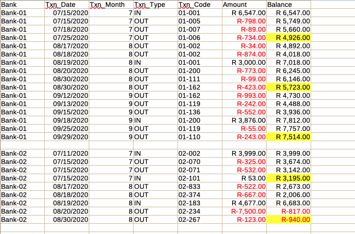
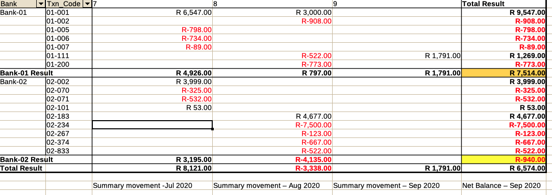
This is another approach using PIVOT TABLES.
Restructure the detail data columns like this
Notes:
- Bank is the bank account number
- Txn_date is the date of the transaction
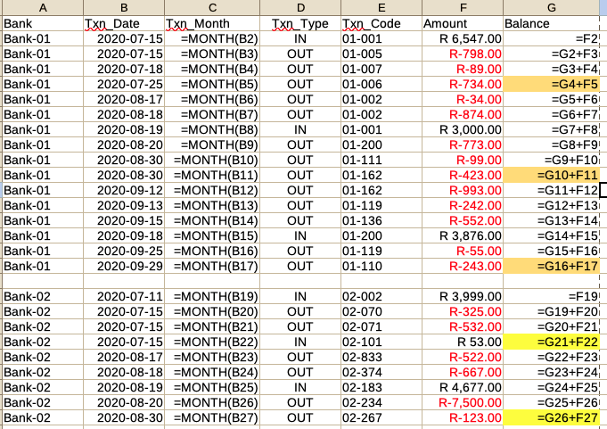
- Txn_Month is determined using the MONTH() Function and copied across all rows.
- Txn_Type groups Receipts (IN) and Payments (OUT)
- Txn_Code is just the transaction allocation codes (example codes)
- Amount - for receipts this should have a positive value and for payments a negative value (the net sum of these will give the monthly net movement and each months monthly net movement total will then be added to provide the selected months total - in the pivot table)
- Balance is the running total - for cross checking purposes
These are the formulas(e)
Select all the cells and
Insert → Pivot Table
Drag fields from the Available Fields to the respective layouts as shown here
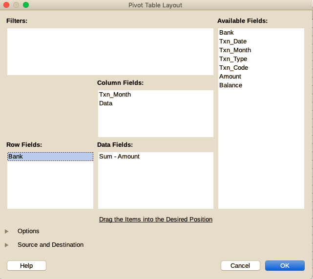
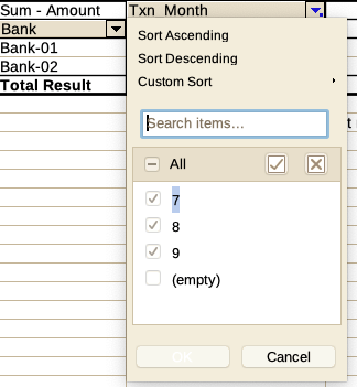
Filter by Txn_Month
Here we are selecting ALL discovered months - excluding the blank row.
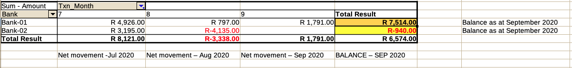
This will give you something like this for July to September 2020
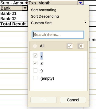
Filter out September 2020 (uncheck 9)
and this would be for the period July to August 2020
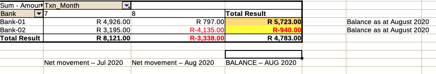
This pivoted table is another cross check of the balances, using the txn_codes to reconcile the transactions that make up the balances.
Sorry about all the screenshots, as I am unable to upload any files at this early stage of my ‘karma’ - not yet received the necessary 5 points 
Thanks for that!