Track asset amount over time

[cabin-74]

Hello,

Here is an attachment of what I have so far. (in case it helps)

question-track-assets.ods

I have a spreadsheet with data with the following structure (dummy data):

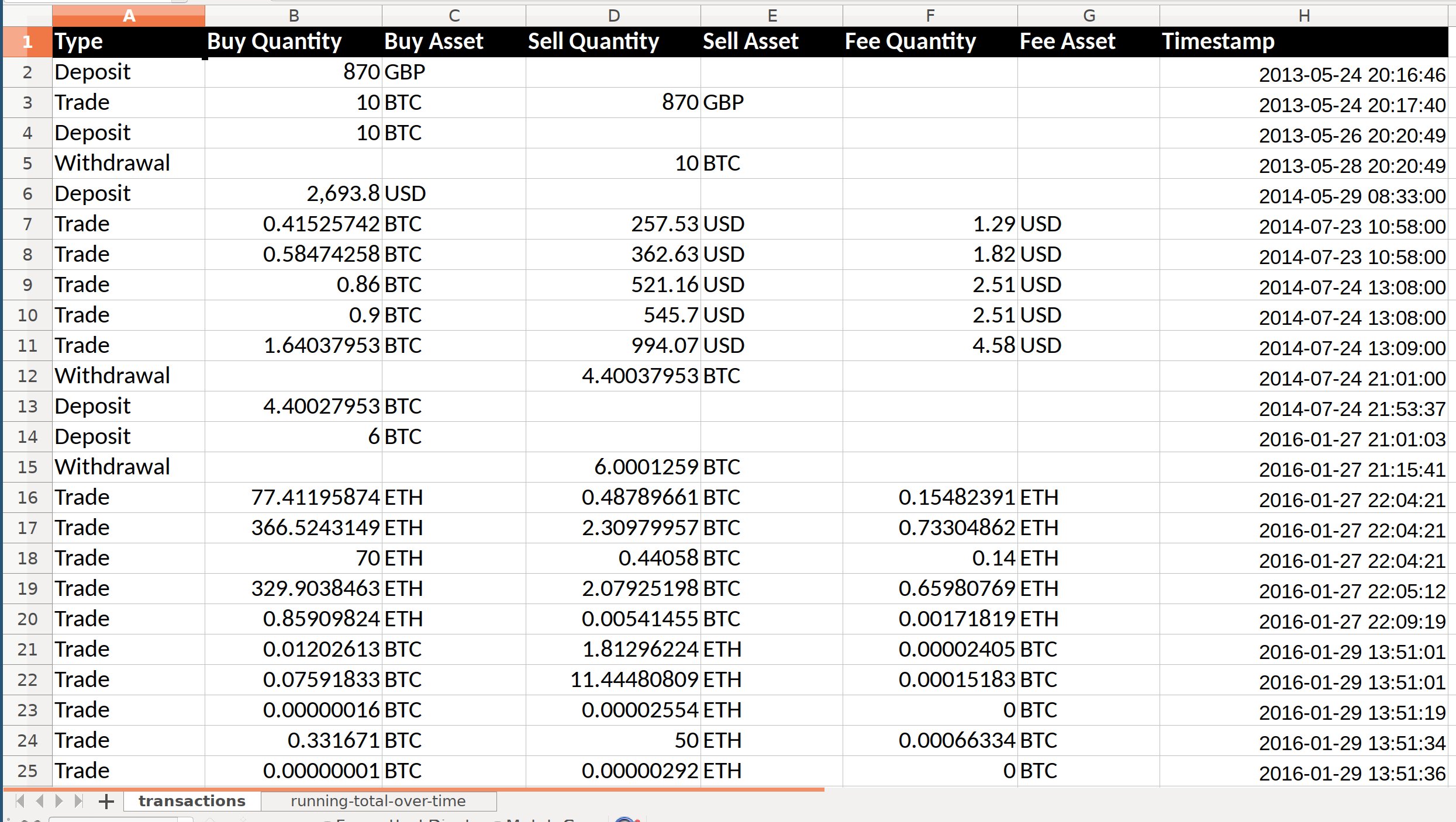
Type Buy Quantity Buy Asset Sell Quantity Sell Asset Fee Quantity Fee Asset Timestamp

There are 3 types:

• Deposit (adding to asset amount)
• Trade (both adding and taking away from assets)
• Withdrawal (taking away from asset)

My Goal:

With the data I have, I would like to create a new sheet which tracks the total amount for each asset on any given day of the year (including days where the asset number held stays the same ie: I want 365 rows showing a running total of how many I have on that particular day.)
So this new sheet would have each day of the year going down the ‘A rows’, then each unique asset from sheet one would have its own column tracking the amount owned on each day.

Here is a mockup of want I’m trying to achieve:

I have no idea how to do this as I’m a complete newb to spreadsheets.

Any guidance or help would be great as I’ve really spent so much time on this and can’t think of a way to do it!

Thank you

[anon73440385]

Hello,

please see the following sample solution:
TrackAssetsModified.ods

To make the formulas

• shorter and more readable
• adaptable to future changes of number of rows in sheet transactions
• or adaptable for performance reasons for lower row numbers in sheet transactions

the sample file implements Named Ranges for each column of table transactions (see Sheet -> Named Ranges and Expressions -> Manage)

The formulas being used look like this one (example is for the BTCvalue at date in cell A2):

=SUMPRODUCT((T_B)*(T_C=B$1)*(ROUNDDOWN(T_H;0)=$A2))
+SUMPRODUCT((T_D)*(T_E=B$1)*(ROUNDDOWN(T_H;0)=$A2)) 
+SUMPRODUCT((T_F)*(T_G=B$1)*(ROUNDDOWN(T_H;0)=$A2))

(adapted for better readability here)

Hope that helps.

[cabin-74]

Wow! Thank you so much Opaque!! There is so much I have learnt from looking at your elegant solution.