Calculate difference between columns in report (pivot table?)

[GWolf]

Hi,

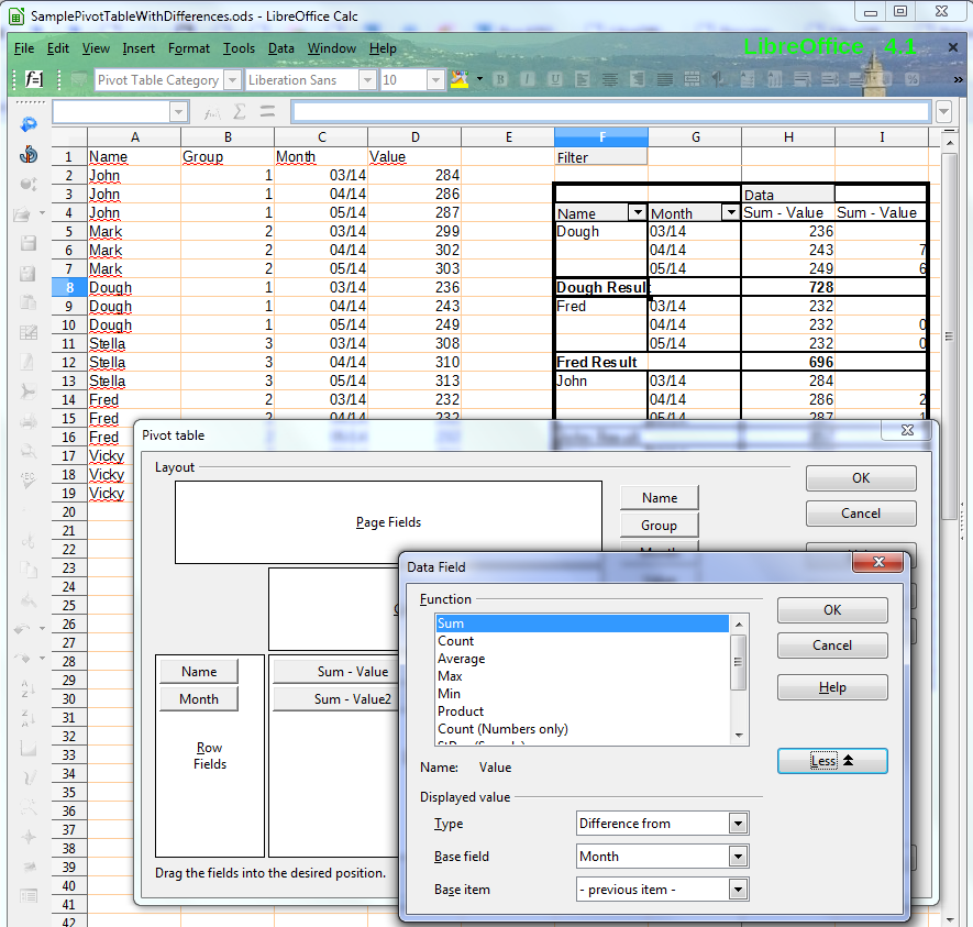
I can not get my head around seemingly simple problem. Suppose I have the following data in Sheet (this is much simplified example, see below). What I want to do is create a report that would have difference compared to previous month per each person/Name, I do not need no sum totals, just difference compared to previous month. In future I would need to create a monthly report each month. Ideally I would also want to filter by Group at some point. I tried Pivot tables, but there just seems no way I can get it done with my current knowledge.

Maybe it is not job por Pivot tables at all? Maybe I can get this same thing done different way, the only requirement being I do not mess with data in original Sheet.

Data:

Name    Group   March   April   May
John    1       284     286     287
Mark    2       299     302     303
Dough   1       236     243     249
Stella  3       308     310     313
Fred    2       232     235     238
Vicky   3       316     318     320

[dajare]

I’m very much an amateur when it comes to Calc, but you can try the sample file, attached (populated with your data), for one solution:

1. (Based on code found at Ask.metafilter.com.) Find the last number in the row, and subtract from it the next-to-last number in the row - using (in pseudo-code):
   INDEX(FirstCell:LastCell,COUNTA(FirstCell:LastCell)) to reference the cells. I put these in a new column C, between group and months (which I expect are going to extend). I subtracted, because it looks like your “norm” is get bigger values month on month.
2. Reference those values in a second sheet to make your report easier (could be skipped!).
3. Set up pivot table between “Group” and “Last Month Diff” columns. Each month, update the values in the pivot table by right-clicking on the table, and selecting “Refresh” from the pop-up menu.

Hope that helps. There is probably a better way to do this, but my sample file (below) is at least working … and I learned something, anyway.

Attached sample file: Diff_to_previous_month_example.ods

[GWolf]

David, thanks, thats at least a start. But I am not entirely sure why there is a SUM() in formula calculating the difference. To me it seems, that instead of =SUM((INDEX(D2:AAB2;COUNTA(D2:AAB2))-(INDEX(D2:AAB2;COUNTA(D2:AAB2)-1)))) it should suffice to specify =INDEX(D2:AAB2;COUNTA(D2:AAB2)-(INDEX(D2:AAB2;COUNTA(D2:AAB2)-1))).

[dajare]

Yep, =(INDEX(D2:AAB2,COUNTA(D2:AAB2))-(INDEX(D2:AAB2,COUNTA(D2:AAB2)-1))) will do it. I did warn you I’m an amateur! Otherwise, it seems to work fairly well.

[mariosv]

@dajare answer it’s fine if you want maintain the data as you have.

The way to do it with Pivot Table is having the data tabulated, one value one record, how you have the data seems a report from row data.

Next a sample file on how organize data to do it with pivot table:
SamplePivotTableWithDifferences.ods
so it’s possible filter the fields by month or name or set up a general filter.

Editing the pivot table and double click on data field to set up for differences.

[dajare]

That’s some serious pivot-tabling! B-) I assume you have the pivot table on the same sheet as the data simply to illustrate? Otherwise it’s hard to see how data is added on this scenario. But if that assumption is correct, this looks extremely versatile. Thanks!

[mariosv]

Your assumption is correct, because it’s not possible insert/delete rows/columns in the area of the pivot table, but sometimes like this is useful.

[GWolf]

I had also had this idea of transposing my data as marisov, but it seemed unnatural to my mind. Anyway, thanks for this example! I will have to reconsider my data arrangement.