I have a spreadsheet file with three sheets: “Holdings”, “Quotes” and “Monthly”.
On Holdings, I have data about stocks I own:
- Column A - Stock symbol
- Column B - Buy Date
- Column C - Sell date
- Column D - Quantity
- Column E - Buy Value
- Column F - Sell Value
- Column G - Value now (
=IF(F2>0, 0, VLOOKUP(A2,Quotes.$A$1:$C$429,3,0)*D2))
On the second sheet (Quotes), I have the prices for all relevant stocks:
- Column A - Symbol
- Column B - Date
- Column C - Price
On the third sheet (Monthly), I would like to get an idea on how the stock was on a set of months:
- Column A - Date (end of month)
=EOMONTH(DATE(2014, 3, 1), 0)for A1 and=EOMONTH(A2, 1)for A2 and on - Column B - Total
My problem is in getting the formula for the column B on the third sheet (Monthly). If I add one column for each stock, I can get the individual values using INDEX(...MATCH()...), but this has some problems:
- Couldn’t get the “sell date” to work on this situation, ie, couldn’t skip the calculation for the month of April if a stock was sold that month
- For each new stock, I would have to add a new column.
- For each new month, I have to copy and manually change the formula for each column (ie, each stock), as it says “the arrays have to be worked together” or something like this, resulting in Err504 if I just drag the formula.
What would be a proper way in getting the totals for column B on the third spreadsheet?
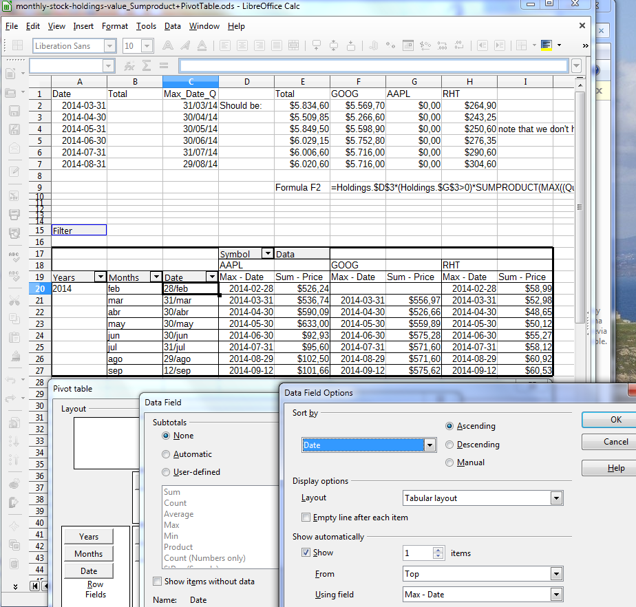
I made a sample spreadsheet is available for download . In the last sheet, I’ve added the expected values on the column D, with the columns E to G with the values per stock.