Calc: How To Remove Both First Occurence and Duplicate Entry From Column

Hi folks,

I would like to know if the following is possible with LO as per the title:
How To Remove Both First Occurence and Duplicate Entry From Column

To make it more clear, here’s an example of what I mean/want to do:

I have one column of words in calc.
The column contains duplicate entries.
What I want to do is remove BOTH occurences where a duplicate occurs, e.g.

column contains:

cat
cat
dog
dog
rabbit
rabbit
goat

when filtered,
I want a column to contain just the non-duplicate word i.e.
goat

As you will see this is NOT the same as removing duplicate entries, as this gives:
cat
dog
rabbit
goat

which is no good in this case.

The answer may be here already or on the web, the problem is being able to find it, so if anyone knows the answer or can point me to it via a link, it would be much appreciated.

Thanks for your time guys :slight_smile:
Tim

Running Win 8.1
LO
Version: 4.2.1.1
Build ID: d7dbbd7842e6a58b0f521599204e827654e1fb8b

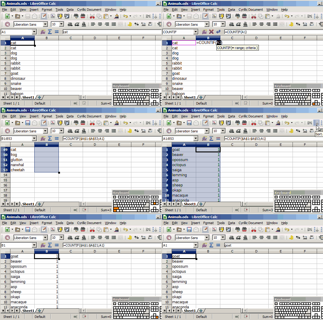
Just add to the next column a simple formula like as =COUNTIF($A$1:$A$70;A1) and sort table by value on it.

Unique values (result of formula equal 1) will be in a few first rows.

Now you can delete other rows or separate data between some sheets or something else…

Remove non-unique values

Hi JohnSUN
I appreciate your reponse, but I’m not an advanced user and don’t know how to do as you suggest
Could you expand on your answers with a bit more detail, i.e. how to.

Am I to use the standard filter or Function wizard?
I tried both with the example =COUNTIF($A$1:$A$70;A1) and just get errors or a blank column.

Thanks for the image Johnsun
but its moving to fast and I cannot follow whats going on.

I have got the basic idea, but unlike in the diagram above, when I enter the code in column B, LO switches it into column A1 and deletes the text entry that is there.
I kind of got it working because it counted the right number of entries for the first 5 duplicate items but then it just repeated 5 for the other words of which there were 2,3,4 and 0 duplicates so I guess I’m doing something wrong somewhere.

Additionally to the correct answer of @JohnSUN:
You can also filter your Data with Criteria: … next Columnequal to1

Hi karolus,

thanks for your reply, but its all Greek to me I’m afraid :slight_smile: can you expand?
see my answer to Johnsun

I still need to be able to do this.

so I have used a video screen capture on the GIF above so I can follow it , unfortunately my keyboard has different layout, anyway

Here are the steps written down that I hope are correct:

  1. All multiple text entries are in column A

  2. Select cell B1

  3. Type in =COUNTIF()

  4. Select cell A1 with left arrow key (makes pink outline)
    4a - In the GIF above it appears that the cell selection A1 -A53 automatically goes between the brackets as they are selected, this is not the case the cursor needs to be placed between the brackets
    In this example the formula should look like this =COUNTIF($A$1:$A$53;A1) note the position of the brackets

  5. Press Ctrl + Shift + down arrow to select remaining text cells in A1

  6. Press Shift + F4 (this adds $ formula to COUNTIF)
    6a Press semicolon key that’s one of these ; (period - comma)

  7. Press Ctrl + home to select cell A1 again

  8. Press enter - Column B changes to entry count of first duplicate words in column A

  9. Press up arrow

  10. Ctrl + Shift + End

  11. Press Ctrl + d

  12. Press Ctrl + home

  13. press right arrow (B1 cell)
    14 Use Sort by column (cannot see data - sorts least to most
    15 Delete all cell numbers (words) with two or more entries, leaving just those with one, the non duplicates.

I would appreciate any correction and will amend this post for others.

Thanks for your time guys.

Thank you for your work! I was looking for ways to comment actions in the animation, or at least slow it. After 6 press semicolon ; - separator parameters in formula, than 7-8-9. Step 10 is Ctrl+Shift+End

Hi Johnsun,
Thank very much for returning to correct me, I will edit the list and add the corrections.
However it is still not working for me as per the GIF.
After step 6 - (Shift + F4)
I added the semicolon as you suggested
selected A1 which then gives… =COUNTIF($A$1:$A$12;A1)
but when I press Enter I get error 509 in column B1
have I missed something?
P.S.
For screen capture video recording
try Jing (basic version is free (records 5 minutes at a time)

"509 - Missing operator - Operator is missing, for example, "=2(3+4) * “, where the operator between “2” and “(” is missing.” (Help). But I see that formula is correct! Tim, can you create small example with this error and attach it to your question?

Hmm,
I have just noticed something, Johnsun, is the LO version on the GIF an old one?
My version is 4.2.1.1
The reason I ask is this: When =COUNTIF() is typed in column B1 and then cell A1 selected A1 appears outside the brackets ()A1, I would say this wrong yes?
Anyway even entering the exact formula manually =COUNTIF($A$1:$A$12;A1) + Enter it still 509’s
Sorry I don’t understand about adding operators, it works in the GIF as above right?

I just rechecked for 4.3.7.2 - also works.

Dang this is a nuisance, I’ll try updating
Ok thanks, at least that eliminates that possibility, it’s curious though as to why my version is behaving differently.
Dang this is a nuisance, I’ll try updating see if that makes any difference.
another thing I have just thought of is that I am not using LO default settings, I’ll look into that too.

Yahoo! Success
After much farting about I got it to work. :smiley:
I’m going to amend the post above to reflect what I did

I knew you had it right JohnSUN, the darned thing just wouldn’t work for me!