Conditional Formatting Fictional Dates

Hello,

I’m a complete beginner to calc, I’ve tried to search up related topics for sorting this out but have so far failed.

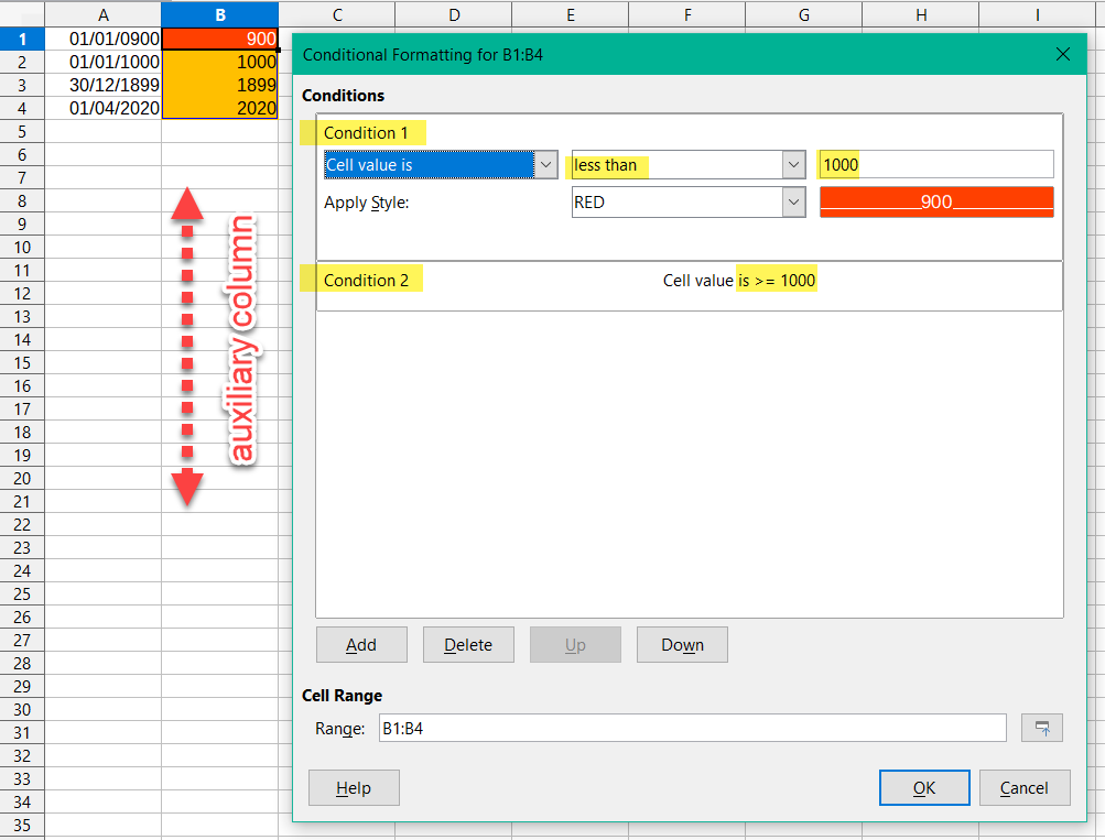
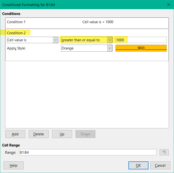
I have some dates, fictional dates, that I want to automatically fill with a certain colour depending on what year is written in it. For example 01-01-1000, below the year 1000 I would want red, but anything above that year orange.
I’m not sure if this is clear enough, or if it’s possible to do it in this way

Don’t use stubborn date fornats. Use ISO 8601 (code in LibO YYYY-MM-DD).
(This is not part of a solution, but a general hint.)

I can only recommend that you work with an auxiliary column and use the year. In the example, the auxiliary column is column “B”.

For “Red” and “Orange” you should create a corresponding style beforehand.

For the solution by @Hrbrgr it is sems assumed that the dates are represented by numbers as it is standard in spreadsheets. If they are given as texts you need to mention that.
In addition: You can also use the Formula is’ mode of ConditionalFormatting.
The conditions would then read YEAR(A1)>=1000 and YEAR(A1)<1000. In this case the second condition is the logical alternative of the first one as far as there is suitable content at all. It could therefore be omitted if the preset color of the range is the wanted orange. Otherwise it might be replaced by ISNUMBER(A1) which excludes the third case: “No entry in that cell”.
Anyway the helper column would then be obsolete.

@Lupp thanks for support.

Or just put 1000-01-01 into a cell (which should make it date); format it as number and see that the serial datetime value is -328711; and use the condition like Cell value is less than -328711.

@Lupp
Thank you so much for writing about the YEAR formulas, it solved my ‘problem’ completely. I just added another condition to keep the empty cells blank and its perfect. Thanks for correcting me on Libreoffice’s year format too.