I’ve been using Calc to sort lists of movie titles alphabetically. Is there any way to set up Calc to ignore “The” or “A” at the beginning of a title? If not in Calc, how about Writer? Either would be fine with me.
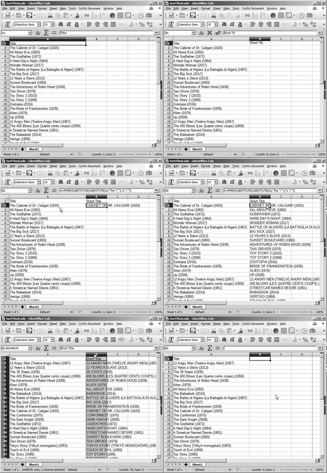
The fastest and easiest way that comes to mind is an additional auxiliary column with a formula like as (if titles in column A of Calc spreadsheet)
=UPPER(SUBSTITUTE(SUBSTITUTE(A2;"The ";"");"A ";""))
Then sort the list and delete this column
Perhaps this animation will help you

(At that point in the film, where one formula becomes a full column, an explanation is needed. Move the cursor to the bottom right corner of the cell until the cursor becomes a crosshair and double-click.)
Same thing here. I need detailed, step by step instructions on how to do this. Assume I’m a total idiot (which is pretty close to the truth here; I have ADHD and being old doesn’t help).
No, no! Not idiot!  The first time is always difficult
@ JohnSun LOL! Actually, I’ve learned to use that expression to get across the point I need simple, detailed, instructions that do not assume I know anything. I’m not an idiot (although I know plenty of people who will debate that point) but there is still a lot I don’t know, including what most people assume would be basic knowledge. It’s the one missing detail in my knowledge, no matter how tiny, that will get me every time.
Your animation was hard for me to follow (thanks to my ADHD, not the animation) but I eventually sussed it out. The “detail” that got me was I had to select the columns with CTRL A instead of just CTRL clicking the two columns. Once I figured that out, I was home free.
The only glitch was one movie, “The 'Burbs” wound up being first because of the stupid apostrophe. For only one title, it was easier for me to copy the contents of the cell, delete that row, insert a row in the appropriate place, and copy the cell into the new row rather than try to horse around with the formula. I also discovered I had to include the cells with title and short title to avoid losing a movie title, then delete them afterwards.
@LadyFitzgerald I congratulate you on this victory! (Thanks to you and Wikipedia, I now know a new word - ADHD, it was new to me. That’s how we learn all the time)
That question has been asked previously on AskLO here.
A quick search with The Duck turned up this solution, which may be what you need:
You would need a help column that will
remove these characters (the and a);if
the list starts in A2 you can use this
in B2=IF(LEFT(A2,4)="The ",SUBSTITUTE(A2,LEFT(A2,4),""),IF(LEFT(A2,2)="A",SUBSTITUTE(A2,LEFT(A2,2),""),A2))copy down as long as needed and sort
by the help columnthe above will take care of A and The
If this answer helped you, please accept it by clicking the check mark  to the left and, karma permitting, upvote it. If this resolves your problem, close the question, that will help other people with the same question.
Only two minor remarks: there is not extra space in "A " and in SUBSTITUTE() easier to use "The " and "A " than LEFT(A2,…) (less to write)
Mea culpa - I was lazy and simply copy-pasted without checking. Your solution is much more elegant.
Thanks, guys, but I need really detailed, step by step, instructions on how to do this. You all are assuming I know something about Calc (or Excel) and I really don’t. I was unable to understand how to do this and my attempt to do so failed miserably.
Then you need to describe to us exactly how your spreadsheet is designed if you need detailed instructions. BTW age doesn’t count as an excuse for not being able to do this stuff - I am for example over 70  Perhaps you could add a (simplified if necessary) example of your spreadsheet to your original question.
I’m going to make myself a tutorial for all this since, at my age, the only thing I retain well is water.
Thanks for the help, everyone!
