How to reverse the icon sets of conditional formatting?

[pinkflowers]

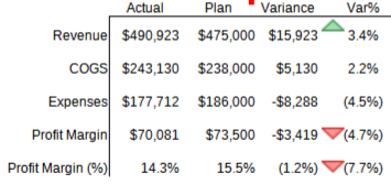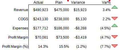
How can I get the icon set for COGS and Expenses to be the reverse rule of how it works for Revenue and Profit Margins?

Revenue, etc. condition used in screenshot: Yellow dash: >= 0 Value. Green up triangle: >= 0 Value.

[joshua4]

There might be a way using the Formula option for each entry under your Icon Set, but I’m having no luck there.
A workaround would be:

1. Say your Var% Revenue cell (3.4%) is E2
2. Insert a column before your Var%, so that is now column E and Var% is column F.
3. Make the entries of the new column switch signs as needed. So E2 is =F2 but E3 is =-F3.
4. Add your conditional formatting to the new E column cells using the exact rules you have been.
5. Format Number on the new E column cells to ;;; This will make the values disappear. So, that’s Format>Cells… then Numbers Tab and Format Code as ;;;
6. Adjust the width of the new E column to just as wide as the triangles plus a little for other systems if you share the document.

[pinkflowers]

Thank you. That did result in something like the look I was going for.

A very creative solution.