I need my inventory sheet to skip blank cells

[Nixie]

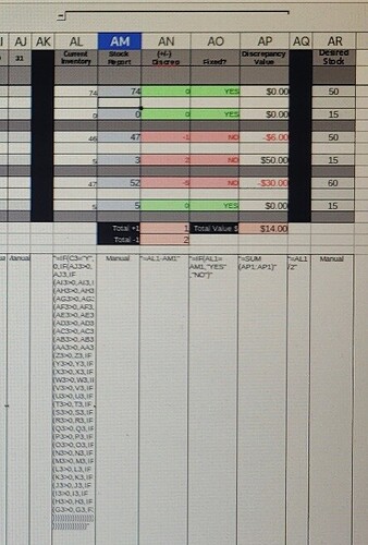
I have created an inventory sheet that has a manual input for our daily inventory.

I want to have a “current inventory” collumn. That can be used to calculate discrepancies daily. (column “AL#”)

My current system is working backwards from the 31st day to the 01st day of the month. (columns “F#”:“AJ#”)

There is an “Out of stock” column where a “Y” is input manually when we are out of stock (column “C#”).

So the current formula goes:

=IF(C5=“Y”,0,IF(AJ5>0,AJ5,IF(AI5>0,AI5,IF(AH5>0,AH5…etc

The manual input of the “Y” is killing me and I know there has to be a way to do =(IF(IS BLANK(AJ3)…etc backwards but it will always calculate the last day and nothing more.

Is there a formula where I can basically have the most recent input showing that is 0 or greater while still skipping the blank cells (they get recorded as 0 in calculations) and while also not having to manually input Y in out of stock.

I know there’s a better way, I just don’t know how.

[joshua4]

Inventory has three dimensions at least: Item, Count, and Date. There are sometimes more dimensions, such as in clothing stores that have a sizing range or color range for a given SKU. In any case, spreadsheets are two dimensional, and are not the right tool for inventories. Have you considered creating a simple database in LibreOffice Base?

That said, having 31 nested IF’s is not a good approach, and is almost certainly unnecessary. I think what you would have better luck at is to post your example spreadsheet as an upload here (edit your original question), then detail what you want in the end without bothering much with what you have done so far to get there. In fact, even creating a hand “faked” example spreadsheet that shows several cases as they ought to appear might be a thought.

In this way you might get a lot more interaction from the community.