Hi, I have a list of things to do. I update the list with the date I completed the tasks.
I have a column full of dates and also another column that lists the frequency (weekly, monthly etc.)
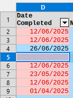
I would like the text colour of the cells containing a date to change colour depending on how many days have passed since that date; they would turn red if 7 days have passed etc.
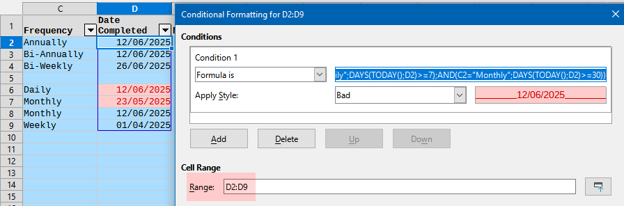
I tried to format the cells using a Condition, e.g.:
Format, Conditional, Condition
Condition 1
Formula is:
DAYS(TODAY(),A1)>=7
Apply Style: Bad
So the above will colour any date past 7 days of the current date; then I change the formula for tasks that are monthly/annually etc.
It works great, but I have to specify the cell reference and frequency for each condition.
In the list are several items e.g.
Task	Category	Frequency		Date Completed
TaskA	Category1	Daily			12/06/2025
TaskB	Category2	Monthly			05/06/2025
TaskC	Category1	Monthly			12/06/2025
TaskD	Category1	Annually		12/06/2025
TaskE	Category3	Bi-Weekly		20/05/2025
Sometimes I add a task in the middle of the list, or use a filter to organise by category. Each time I add a new item I have to manually enter the cell reference etc.
Ideally I think I would need a formula that also uses the Frequency column (I could change this to a number, e.g. 7 instead of ‘weekly’ to keep things simple).
Then, hopefully I could use just one Condition across all the dates.
I am hoping someone may be able to help?
Edit: I have attached a sample file:
sample.ods (15.4 KB)