LibreOffice Calc - total distance per shoe

I wish to add onto numbers in a column which match text in a different column.
In this instance it is to keep track of the total distance I have run in various shoes.
Example screenshot is attached.
total per shoe

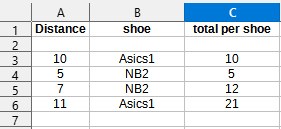
A bonus would be hiding older totals. In the attached case I’d only see the 12 and 21.

You can upload the file here so someone can look at it and figure out how the calculations are done so far. Thank you.


…older totals.

You mean older than yesterday, last month, last year. Do you use a date for your entries?


Which operating system and LibreOffice Version do you use?

The bonus thing may be tricky. The idea was that I would only see the cumulative total distance for each shoe. So in my example, when I used each shoe for the second time, the first total would be hidden (white text?).

Yes I have a date column. Each new date goes in the next row down.
[
distance example.ods (26.8 KB)
Example file attached. I’ve coloured the cumulative totals that I want to see / or emphasise]
Version 7.3 on Windows 10.

Here is an “obvious” take based on “normal” ways to accumulate values from a list. I don’t know if the formatting is what you want or not.

What we are doing here is using the SUMIF function keyed from the columns that you have. There are no old values shown in this case, just the current total for each shoe…errr…probably pair of shoes.

Shoe Distance Accumulators.ods (16.0 KB)

Thanks Joshua4.
That is the data I want, so I will use that to start with.
My sheet will have hundreds of rows, so I don’t want the data to be fixed in position. I’ll experiment with cut & paste to move it down every so often.

Or consider putting it up at the top as far as it can go, then using the Freeze Rows feature.

  1. Select all of the results part, including the headers.
  2. Slide it so that the top header is in row 1.
  3. At the far left click and drag to select the 1,2,3,4 row labels. (Make sure you aren’t seeing a double-headed mouse pointer when you start dragging, just a single-headed one).
  4. In the menu bar click View>Freeze Rows and Columns.

If you want to be pretty about it, you can first insert three empty rows at the top so that you don’t always see your first three days of data. It will act just like the title of this question acts here on this website.