Yes, your task is easy to solve. But you need to slightly expand the set of functions of Calc with the help of this extension - ListOK
After installing this extension in the Add-In category of the Function Wizard, several additional functions will appear, the names of which begin with LST
All of them are designed to handle lists of natural numbers, exactly as shown in your screenshot.
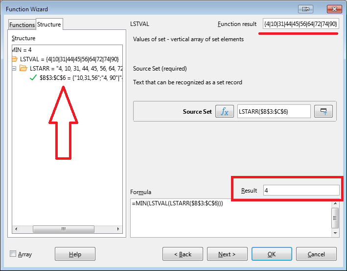
The LSTARR() function will collect all values from the specified range into a single list and for your cells it will turn out 4, 10, 31, 44, 45, 56, 64, 72, 74, 90. This is a string, it is simply impossible to apply the MIN() function to it, as pointed out by a respected colleague of @Zizi64.
Therefore, use another function provided by this extension - LSTVAL(). Its result is an array of numbers that go into the string. The MIN() function can be applied to this array and for your example we will get the result 4
The LSTIN() function will check each cell - is 4 in the list of values for this cell? Apply conditional formatting to the range of your cells and hilight the cells with the minimum - the problem is solved
Update. After discussing the solution with distinguished colleague @mikekaganski , I came to the conclusion that I misunderstood your desire as stated in the question. To find the cell with the minimum value in a row, the formatting condition must refer not to the entire range, but only to the cells of the current row. That is, the formula should be like this
LSTIN(MIN(LSTVAL(LSTARR($B3:$C3)));B3)
or even like this
LSTIN(MIN(LSTVAL(LSTARR(3:3)));B3)


