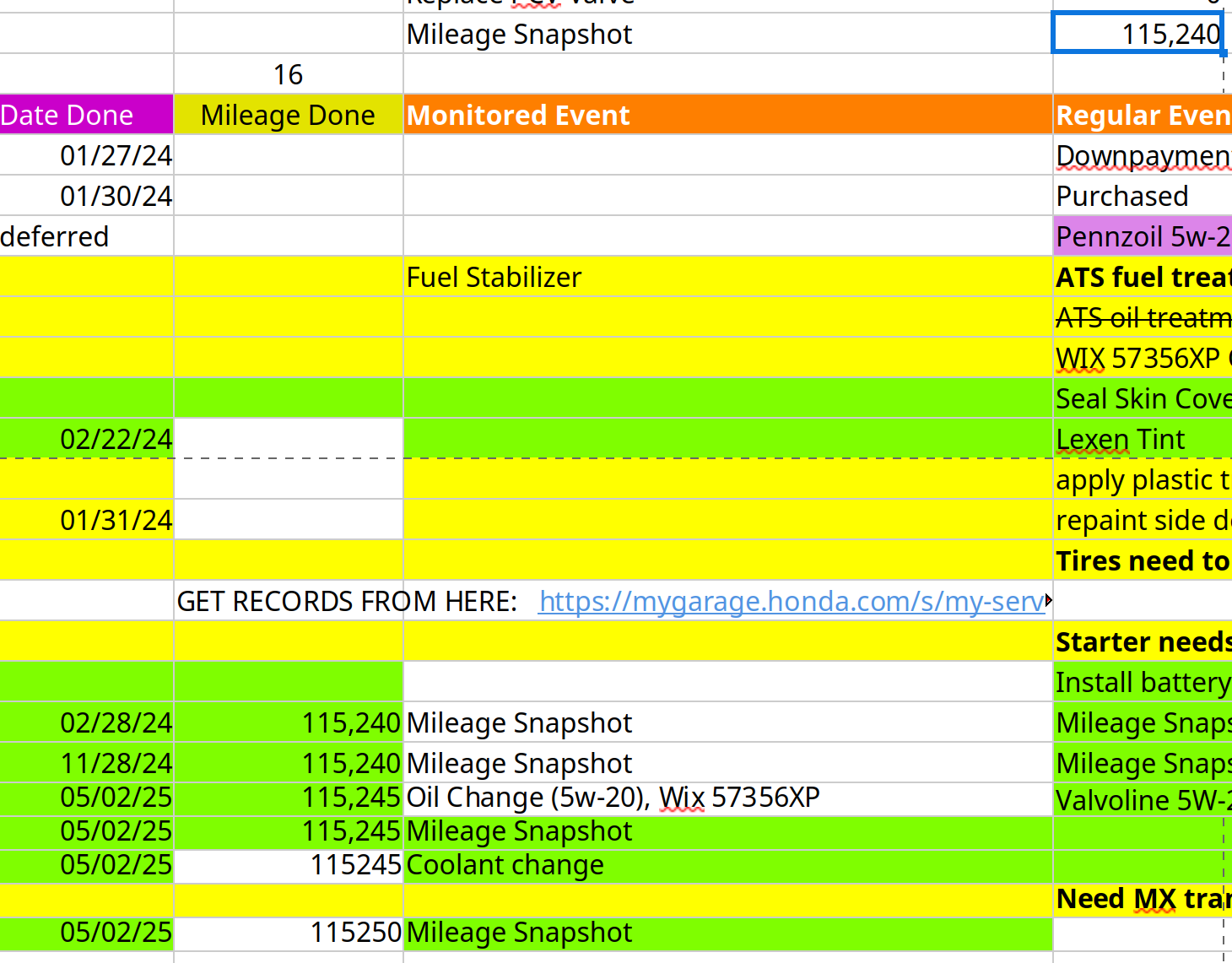
I am trying to upgrade my car maintenance spreadsheet so that it has a dashboard showing what is coming due and what is overdue to routine maintenance. All dashboard functions depend on returning the value of an adjacent cell relative to the last row that contains an occurrence. For example, in the screenshot below, the dashboard item “Mileage Snapshot” (selected cell) should retrieve the Mileage adjacent to the last row (cell) that contains the string “Mileage Snapshot”.
Based on reading many posts, I was able to come up with this formula.
=OFFSET($B$27,(MATCH(C24,$C$27:$C$499,-1)-1),0,1)
However, the function MATCH doesn’t return the last occurrence, it returns the first matching occurrence and according to the docs, depends an assumption of sort order. That’s a problem because as you can see in the example, the last Mileage Snapshot in the event list occurs at 115,250 miles but the function above returns 115,240 miles.
How do I get Calc to return the last occurrence of a matching item?