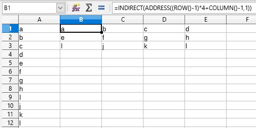
I want to take a column of 120 or so numbers from a spreadsheet and enter them in another spreadsheet in 4 columns.
So, the first 4 numbers would be side by side in row 1 and the second 4 numbers would be in row 2.
I have a workaround that is doable but labor intensive. I can highlight the first and 5th and 9th etc. numbers until I get to 117, and then Copy or Cut and then Paste into the new spreadsheet.
And repeat 3 more times.
I think there should be someone out there who has already figured this out.
If not, maybe I’ll need to learn how to write a Macro.
What was wrong with the formula @jimk posted? It works flawlessly for the pupose. You won’t find a ready-made tool for the very specific proceeding.
I didn’t see it yet. Just now I hit the refresh button in my URL field and got these messages.
It does work flawlessly! It is the answer to my needs. I couldn’t have ever figured out how to write that equation. Awesome!
I didn’t see until 10 minutes ago. It does work flawlessly. Thanks @jimk.
I do not see where I can thank him except in these Comment boxes.
You’re welcome!
The way to thank someone is to mark the answer as correct, which you have done, and consider upvoting the answer (maybe you did this too; it’s anonymous so I’m not sure). Optionally add a comment, which you have also done. It would have been more proper to comment on the answer, rather than the question, but that’s a minor point.
I looked there but thought that it would be commenting on the comment about commas and semi-colons.
Enter the following formula in cell B1.
=INDIRECT(ADDRESS((ROW()-1)*4+COLUMN()-1;1))
Then drag to fill over to E1, then down as far as needed.

Finally, cut from columns B through E and paste special as values into the new spreadsheet.
A majority of locales cannot use the comma as the parameter delimiter because it conflicts with the decimal separator. The semicolon is still accepted globally by all locales. For some time now it got replaced for the display by a comma in locales using the point as the decimal separator. An ingenious idea to mess up international cooperation in forums.
But you will not be blamed if you continue to post formulas with the semicolon.
Thanks!
BTW, shouldn’t the last word in Lupp’s comment be “comma”?
There is also a way with less and simpler fomulas: Paste the copied column 4 times in adjacent columns, the first one starting at row five, the next one to the right one row higher and so on. Above the first element in the last column you have one empty cell now. Right of the first element in the last row column enter the formula =(MOD(ROW()-1;1)=0)=(MOD(ROW()-1;4)=0) and fill it down for all the non-empty rows. Now select this column completely and choose the ‘Autofliter’ from ‘Data’. From the dropdown of the filter select TRUE. If you now copy what not is filtered out, you can paste it elsewhere to get the wanted result. Hmmm… Lot of handiwork… (Just for completeness, kind of.)
I got as far as the formula into the cell right of the last row. When I filled it down, the whole column said “TRUE”. And then nothing happened using Autofilter.
Sorry! There was a typo. The formula should say TRUE in every fourth row. starting with row 5…
ROW()-1 returns 4, 5, 6, 7, 8 ,9 and so on then, row by row. It’s one of the rows where a valid group of 4 consecutive elements is shown exactly if the number returned is divisible by 4 without a remainder. The MOD function is made for this: MOD(SomeInt; SomeIntDivisor) returns the remainder you get if you divide SomeInt by SomeIntDivisor. Mod(N;1)=0 is always TRUE, of course.
I tried it again with your changes, and it does work. It’s very interesting how different approaches can yield the same result. Thanks.
