
I have a spreadsheet range(31 rows for a month) where I have an overall format based on ISEVEN(ROW) to get alternating background displaying grey rows for easy reading. Within that range I have a column that has a conditional formation with 3 conditions. If the entered number is within a certain range, the cell will either have a yellow, light red, or a dark red background. If the entered number is not in range, then I want the background as grey that was originally apply to be displayed. I tried having the grey background created first before the other formats and after; does not work. I tried applying as a found condition also. In either case, the grey row will appear, but the special conditions will not. If the grey is not applied, then the other colors appear as expected.
Click Format > Conditional > Manage the Manage Conditional Formatting dialogue window opens. If you look at the image below, the formatting in the top row is overridden by the formatting in the following condition.
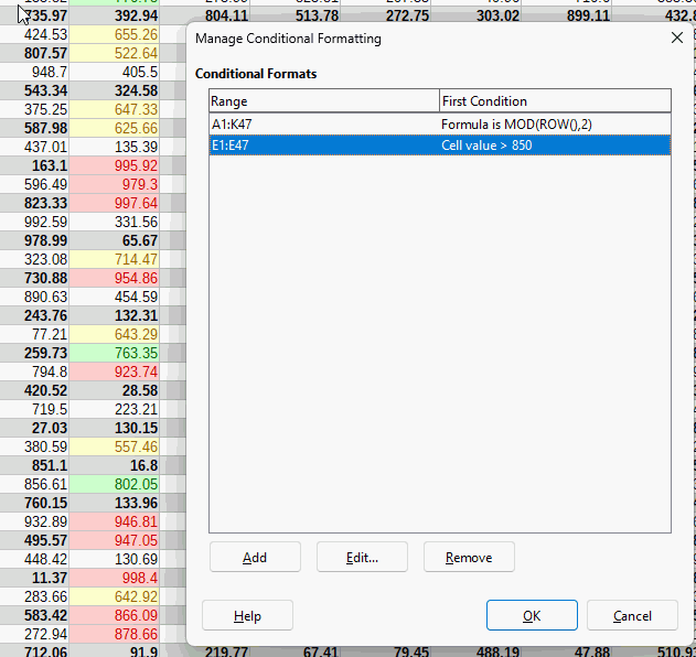
The only way to change the order is to remove an earlier condition (lower line) and recreate it so it goes to the top. There is an enhancement request, tdf#148154 , to allow the conditions to be moved relative to others.
[EDIT]
So the answer to your question is to open the Manage Conditional Formatting dialogue and Remove the alternating rows conditional format and then create it again.
2 Likes
Thank you. Your clear explanation yielded the desired effect.
1 Like