Calc - Sorting text from vertical view to horizontal and grouping

[nobeja]

• For this post I attached image, because I couldn’t format properly text.

Is it possible with pivot table or some other way, without macros and scripts, to sort and group text from this

|Bank 1 50|
|Bank 2 100|
|Bank 3 150|
|Bank 4 23|
|Bank 3 36|
|Bank 1 95|
|Bank 3 56|
|Bank 1 24|
|Bank 2 12|
|Bank 2 58|

to this

|Bank 1 Bank 2 Bank 3 Bank 4|
|50 100 150 23 |
|95 12 36 |
|24 58 56 |

I tried some combination with pivot table, but without success.

[mikekaganski]

Please check if this answer helps you.

[nobeja]

Thank you for suggestion but I couldn’t switch from vertical to horizontal view with decroise extension, it doesn’t sort data the way like it’s on the image. I tried few combination in decroise extension, but without result.

[SM_Riga]

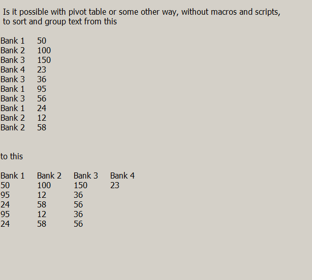
Yes, it is possible. Assume we have such table:

Bank	Amount
Bank1	50
Bank2	100
Bank3	150
Bank4	23
Bank3	36
Bank1	95
Bank3	56
Bank1	24
Bank2	12
Bank2	58

1.Firstly, we need to determine unique “Bank” entries. Select all cells with bank entries, go to Data > More Filters > Standart Filter..., select “Not Empty” value and under Options select No duplications and Copy results to:, then choose where to copy filter result. You will get column with Bank1, Bank2, Bank3 and Bank4 entries:

Unique entries
Bank1
Bank2
Bank3
Bank4

2.Then we need to to match all amounts connected with this bank. In the cell next to Bank enter an array formula (address references from my demo spreadsheet, may differ from yours):

=TEXTJOIN(";";1;IF($A$3:$A$12=D3;$B$3:$B$12;""))

NB! To enter an array formula you need to accept it with CTRL + SHIFT + ENTER As a result you will get:

Unique entries	Amounts
Bank1	50;95;24
Bank2	100;12;58
Bank3	150;36;56
Bank4	23

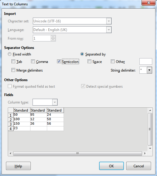
3.Lets split amounts to one per cell. Select all four cells with amounts, go to Data > Text to Columns... and under Separator Options select semicolon as separator:

As a result you will get such table:

Unique entries	Amounts	Amounts	Amounts
Bank1	50	95	24
Bank2	100	12	58
Bank3	150	36	56
Bank4	23		

4.The last step is to transpose this table. Select any free cell and enter an array formula (accept it with CTRL + SHIFT + ENTER), where D11:G14 is a range from previous step:

=TRANSPOSE(D11:G14)

5.And voila:

Bank1	Bank2	Bank3	Bank4
50	100	150	23
95	12	36	
24	58	56	

I have also attached demo spreadsheet - Data_sort.ods

P.S> I am not strong with Pivot Table functionality, I believe there should be even easier solution. I just could not get Data Fields without applying any functions to them.

[nobeja]

Thank you for answer.