VLOOKUP on multiple ranges with tilde?

[DonD]

Running Libroffice Calc v6.2.0.3 on Ubuntu 18.10.

I am trying to use VLOOKUP() with multiple ranges but can’t get this to work.

Following is an example of the sort of thing I am trying to do:

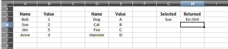
The formula in cell H3 would be: =VLOOKUP( G3, (A3:B6~D3:E6), 2, 0 )

ie: Lookup the value in G3 from both A3:B6 and D3:E6 and return the second column in the matching row.

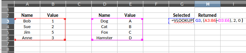
When I edit the formula both the source ranges are hilighted (see below) and everything appears correct, but I always get an Err:504

Have I missed something obvious or am I trying to do something that can’t be done with VLOOKUP()?

(And sorry, no… can’t just move the second range to below the first. )

Any ideas how I can get this to work?

[mikekaganski]

Yes, that is impossible (yet? Please file an enhancement request - but that would be incompatible change).

[erAck]

Please don’t file an RFE, it won’t get implemented, because it’s incompatible in the sense that no other spreadsheet implements it that way and the function is defined to take one range.

[PYS]

Hi

VLOOKUP on multiple ranges with tilde is not possible, but INDEX allows it and it has an argument to work with it.

Unfortunately the MATCH function does not offer this possibility. In the attached example I proceed in two steps: find range & line with MATCH and then the result you are looking for with INDEX.

Regards

[erAck]

So, short answer: No. This is not possible.

[gregors15]

Using the same columns you used, try this…
=IFNA(IFERROR(INDEX(B3:B6,MATCH(G3,A3:A6,0),1),INDEX(E3:E6,MATCH(G3,D3:D6,0),1)),“Not Found”)
Regards