How to alternate row background colors WITHOUT overriding conditional font color

I’d like to have a table in LibreOffice Calc 5.3.0 that has alternating row background colors, and at the same time highlights values below 5 with a red font color. Here’s an example of how I want it to look:

expected result

But I want the styles to be fully dynamic, so that I can modify cell values and add/remove rows and the styles will update themselves accordingly.

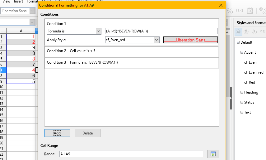
From what I read, it sounds like I need conditional formats - but I can’t get it to work correctly. Here is what I did:

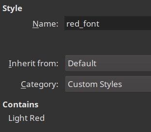
  1. I created two custom cell styles:

style 1
style 2

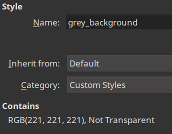
  • Style grey_background has no properties set except for a grey background.
  • Style red_font has no properties set except for a red font color.
  1. I added two conditional formats to the cell range that contains the table:
  • One conditional format applies style grey_background based on the formula isodd(row()).
  • One conditional format applies style red_font if the cell value is less than 5.

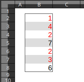
But the result is wrong:

actual result

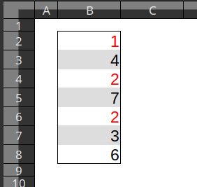
As you can see, the numbers 4 and 3 didn’t turn red, even though they match the “less than 5” condition. It’s as if the grey_background style is blocking the red_font style from being applied to the same cell.

What is happening there, and how can I fix it?

I note the workarounds below, but it is a shame that LO Calc doesn’t feature this, or include a format option that doesn’t require conditional formula use. For comparison, the free (price) competitor Google Sheets does it and this feature produces easy to read/use sheets.

You need one more format for the row with red background and red font.

ConditionFormat_rows+textcolor.ods

So to be clear, there’s no way to let two styles stack?

Manually creating additional styles for each combination isn’t very scalable. Imagine if I’d want 10 different dynamic styles… instead of creating 10 Styles and 10 simple Conditional Formats, I’d have to create 1024 Styles and 1024 complex Conditional formats.

Hi

If I understand the question you only need a user-defined number format:

[>=5]Standard;[<5][RED]Standard;Standard

and only one conditional formating

ISEVEN(ROW(A1))

See CondFormat.ods (use Shift+Ctrl+F9 to test different values)

Regards

Oh, that’s neat. Too bad it only supports these 8 colors though.

Yes you are right but IMHO in this context (font color) the number of shades is less important because more difficult to perceive.