
Hello,
I have again issues with conditional formatting. I want to apply 3 different formats. Depending on the value in the column “R” I want to color the row from “A” to “J” with
- a red background color when the value in “R” is 1
- a green background color when the value in “R” is 2
- a grey background color when the value in “R” is >4
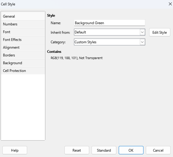
I defined three styles (the background color) and added the first rule as follows:
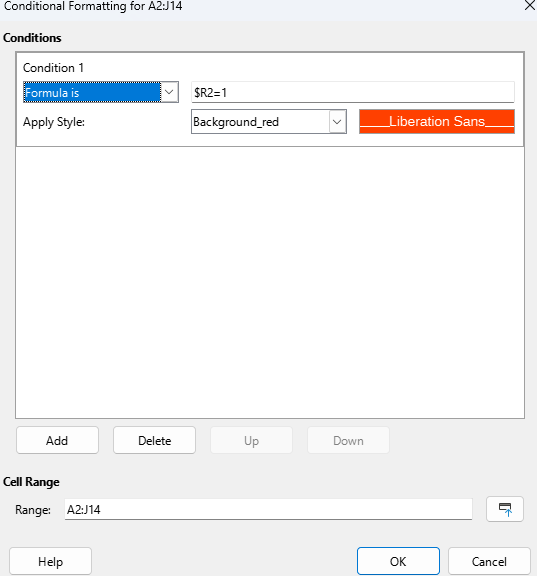
(for rows 2 to 14 to test that rule). But even there are values “1” in column “R”, no row from 2-14 is colored in red. I also tried “$R2==1” but still no coloring of the rows.
What am I doing wrong?
 ).
).