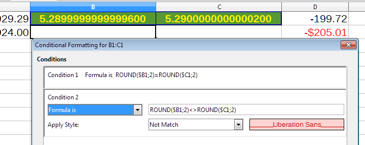
I want to use conditional formatting to color the cell backgrounds of 2 cells. Green when the values match and red when they do not match. The values in both cells are derived from formulas, but even when the values match, the conditional formatting displays the backgrounds as red. How can I make conditional formatting utilize the cells’ values as opposed to the cells’ formulas, which is what I believe they’re using when checking for a match? Sample.ods
Please share a minimal sample file to test.
I’ve attached the sample (I think) above. The cells in question are on Sheet 2, cells B1 and C1.
You don’t get the TRUE value that you expect because these values are really different. Increase the number of digits displayed after the decimal point and you will see this with your own eyes.
As a workaround, you can use the ROUND() function, which will allow you to compare coarser values.
Brilliant! Thank you. I was not aware of the ROUND function. I appreciate the help.
For @rebelstar There was sample worksheet by @Lupp attached in this thread How do I test cell for a whole integer, showing how untrustable (by means of precison) decimal calculations could be. Even 24.24 - 24.00 gives you result 0.239999999999998, not 0.24 as you would expect.

