Extracting time from a huge number in hours

I have this situation, for example:
1
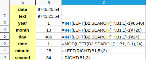
What is shown by these formulas is another interpretation of the date. How can I get the number of months that remain after subtracting the 1 year from the date, and the number of days after subtracting the years and months already calculated?

Also, i tried to concatenate all the values obtained in these cells, but it shows me the #Value! error. The date has a function in the back (SUM), and if i try to introduce the number by hand i get a date and hour type of cell, even though the cell is formatted in [HH]:MM:SS. How can i solve this?
Thank you.
emy1_132308.ods (16.6 KB)

Do you really expect us to rebuild your spreadsheet from a screenshot?

1 Like

Attached.
Never meant that. I thought you can respond from your head, without trying.
Reattached the calc file with the concatenate function.

If you really want this, the only viable solution I can imagine is writing a function in Basic, returning a string to another cell.
Keeping users well aware it’s an approximation, of course.
So, say, for the
251814:04:33 = 10492.25
years = integer part of < this_parameter >/365.25
[…]
and at last you mount the returning string.

Did you read and understand what was posted here?

Repeated in short: Neither months nor years can be used as units in durations because they differ in length. (To a minor extent also days.)
In addition: A day has 86400 seconds (24*60*60 = 24*3600).

If you don’t worry much about exact meaning, you can use the function DATEDIF() which looks to me as if invented by MS. It disregards the mentioned facts, but even this nonsense function doesn’t try to give a reminder in real units.
emy1_132362Re.ods (19.0 KB)

I meant to use the average number of days in a year (approximately), i’m fine with an error of a few seconds.

Your problem is the difference between text and number together with bad formatting.
Select all cells [Ctrl+A].
Remove formatting [Ctrl+M].
Now you see all numbers aligned to the right cell borders and text to the left.
SEARCH(":";B5;1)-1) returns #VALUE because there is no colon in the numeric value of B5.
B6 is a text, indeed. 4 digits, a colon, 2 digits, a colon and 2 digits. B6 is not a formatted number.

Nobody can tell that from a screenshot, particularly not when all cells are formatted to show their content centered.

1 Like

The duration of a year varies not just by “a few seconds” but by a full day (86400s).
The duration of a month varies by up to 3 days.

If you insist on expressing durations using years and months it’s at least a serious mistake to also give a supposed remainder in days and in real units of time.

Use the strange DATEDIF() in mode "y" an "ym" as I already showed you.

@Villeroy
I have obtained something by using only the cell with the text format, but the formula got something like this: 0Y 0M 6D 13H 30M 00S.
How can i transform it into this type: 0Y 0M 6D 13:30:00 ?
Sorry if i’m asking too many questions, but i don’t know everything.

@Lupp
I don’t have two dates, i have an amount of time, so Datediff is not useful in this case.

Times and dates, are numbers.
Enter the decimal 23456.75 into some cell and apply some date-time format. The cell shows 1964-03-20 18:00:00 without changing its value.
With 23456.75 in A1,
=Year(A1) shows 1965
=Month(A1) shows 3
=Day(A1) shows 20
=Hour(A1) shows 18.
Same with formatted number $ 23,456.75 in A1. The cell value is always the same number, no matter how it is displayed.
Day #23456 after day zero (1899-12-30) was March the 20th in the year 1964. 0.75 is 3/4 of day #23456 which gives 18:00.
These day numbers counting days from a given day zero is how all spreadsheets used to represent dates since 4 decades.
SUM always returns a number. SUM(A1:A9) ignores any text values in A1:A9.
TEXT converts any number into a text and returns the textual representation of the given number according to the given format string. If there is a text in A1, TEXT(A1;…) returns that text regardless of the format string.
When you apply functions like LEFT, MID, RIGHT, SEARCH to numbers, these text functions operate on the plain decimal representation of the number. With number 23456.75 in A1, LEFT(A1;5) returns the text “12345”, which is not the same value as the number 12345.